import numpy as npNB: NumPy First Steps
NumPy

A new data structure
Essentially, NumPy introduces a new data structure to Python — the n-dimensional array.
Along with it, it introduces a collection of functions and methods that take advantage of this data structure.
The data structure is designed to support the use of numerical methods: algorithmic approximations to the problems of mathematical analysis.
New Functions
It also provides a new way of applying functions to data made possible by the data structure – vectorized functions.
Vectorized functions replace the use of loops and comprehensions to apply a function to a set of data.
In addition, given the data structure, it provides a library of linear algebra functions.
New Data Types
NumPy also introduces a bunch of new data types.
Python for Science
NumPy stands for “Numerical Python”.
Because numerical methods are so important to so many sciences, NumPy is the basis of what is called the scientific “stack” in Python, which consists of SciPy, Matplotlib, SciKitLearn, and Pandas.
All of these assume that you have some knowledge of NumPy.
Let’s take a look at it.
Importing the Library
NumPy is by widespread convention aliased as np.
The ndarray
The ndarray is a multidimensional array object.
Let’s explore it some.
First, let’s generate some fake data using NumPy’s built-a random number generator.
Note that np.random.randn() samples from the “standard normal” distribution.
# np.random.randn?data = np.random.randn(2, 3)dataarray([[ 0.72834379, 0.5874105 , -0.32733983],
[-0.57066835, 1.08009114, -1.56702285]])data * 10array([[ 7.2834379 , 5.87410495, -3.27339826],
[ -5.7066835 , 10.80091141, -15.67022852]])data + dataarray([[ 1.45668758, 1.17482099, -0.65467965],
[-1.1413367 , 2.16018228, -3.1340457 ]])data.shape(2, 3)data.dtypedtype('float64')About Dimensions
The term “dimension” is ambiguous. * Sometimes refers to the dimensions of things in the world, such as space and time. * Sometimes refers to the dimensions of a data structure, independent of what it represents in the world.
NumPy dimensions are the latter, although they can be used to represent the former, as physicists do.
The dimensions of data structures are sometimes called axes.
Consider this: Three-dimensional space can be represented as three columns in a two-dimensional table OR as three axes in a data cube.
Creating ndarrays
From a list:
data1 = [6, 7.5, 8, 0, 1]
arr1 = np.array(data1)
arr1
array([6. , 7.5, 8. , 0. , 1. ])From a list of lists:
data2 = [[1, 2, 3, 4], [5, 6, 7, 8]]
arr2 = np.array(data2)
arr2
array([[1, 2, 3, 4],
[5, 6, 7, 8]])arr2.ndim2arr2.shape(2, 4)arr1.dtypedtype('float64')arr2.dtypedtype('int64')Initializing with \(0\)s using a convenience function:
np.zeros(10)array([0., 0., 0., 0., 0., 0., 0., 0., 0., 0.])np.zeros((3, 6))array([[0., 0., 0., 0., 0., 0.],
[0., 0., 0., 0., 0., 0.],
[0., 0., 0., 0., 0., 0.]])np.empty((2, 3, 2))array([[[0., 0.],
[0., 0.],
[0., 0.]],
[[0., 0.],
[0., 0.],
[0., 0.]]])Using .arange() (instead of range())
np.arange(15)array([ 0, 1, 2, 3, 4, 5, 6, 7, 8, 9, 10, 11, 12, 13, 14])Data Types for ndarrays
Unlike any of the previous data structures we have seen in Python, ndarrays must have a single data type associated with them.
Here we initialize a series of arrays as different data types (aka dtypes).
arr1 = np.array([1, 2, 3], dtype=np.float64)
arr1.dtypedtype('float64')Note that dtypes are defined by some constants attached to the NumPy object.
We can also refer to them as strings in some contexts.
In other words, in the context of the dtype argument, 'float64' can substitute for np.float64.
np.array([1, 2, 3], dtype='float64')array([1., 2., 3.])arr2 = np.array([1, 2, 3], dtype=np.int32)
arr2.dtypedtype('int32')Integer arrays default to int64:
arr = np.array([1, 2, 3, 4, 5])
arr.dtypedtype('int64')So you may want in use a more capacious type:
float_arr = arr.astype(np.float64)
float_arr.dtypedtype('float64')Arrays can be cast:
arr = np.array([3.7, -1.2, -2.6, 0.5, 12.9, 10.1])
arr
array([ 3.7, -1.2, -2.6, 0.5, 12.9, 10.1])From floats to ints:
arr.astype(np.int32)array([ 3, -1, -2, 0, 12, 10], dtype=int32)From strings to floats:
numeric_strings = np.array(['1.25', '-9.6', '42'], dtype=np.string_)
numeric_strings.astype(float)
array([ 1.25, -9.6 , 42. ])Note that NumPy converts data types to make the array uniform:
non_uniform = np.array([1.25, -9.6, 42])
non_uniform, non_uniform.dtype
(array([ 1.25, -9.6 , 42. ]), dtype('float64'))Ranges default to integers:
int_array = np.arange(10)int_arrayarray([0, 1, 2, 3, 4, 5, 6, 7, 8, 9])We can use the dtype on one array to cast another:
calibers = np.array([.22, .270, .357, .380, .44, .50], dtype=np.float64)
int_array.astype(calibers.dtype)
array([0., 1., 2., 3., 4., 5., 6., 7., 8., 9.])And here is an empty array of unsigned integers:
empty_uint32 = np.empty(8, dtype='u4')
empty_uint32
array([0, 0, 0, 0, 0, 0, 0, 0], dtype=uint32)NumPy Data Types
i - integer
b - boolean
u - unsigned integer
f - float
c - complex float
m - timedelta
M - datetime
O - object
S - string
U - unicode string
V - fixed chunk of memory for other type ( void )
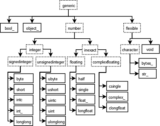
Data Type Hierarchy
NumPy introduces 24 new fundamental Python types to describe different types of scalars.
These derive from the C programming language with which NumPy is built.

See the NumPy docs.
Element-wise Arithmetic
NumPy arrays can be transformed with with arithmetic operations.
These are all element-wise operations.
Let’s start with a 2D array.
arr = np.array([[1., 2., 3.], [4., 5., 6.]])
arr
array([[1., 2., 3.],
[4., 5., 6.]])arr.shape(2, 3)arr * arrarray([[ 1., 4., 9.],
[16., 25., 36.]])arr - arrarray([[0., 0., 0.],
[0., 0., 0.]])1 / arrarray([[1. , 0.5 , 0.33333333],
[0.25 , 0.2 , 0.16666667]])arr ** 0.5array([[1. , 1.41421356, 1.73205081],
[2. , 2.23606798, 2.44948974]])Now let’s compare two arrays.
arr2 = np.array([[0., 4., 1.], [7., 2., 12.]])
arr2
array([[ 0., 4., 1.],
[ 7., 2., 12.]])arr2 > arrarray([[False, True, False],
[ True, False, True]])Boolean arrays will prove to be very useful …
Indexing and Slicing
Example 1
→ Editor’s Note, this jumps ahead to multi-dimensional indexing.
foo = np.random.randn(3,5)fooarray([[ 0.65002831, 0.46012775, 0.83902353, -0.57930057, -0.78375454],
[ 1.29259796, -1.16119504, -0.75869717, -0.39494693, 1.23975995],
[-0.35519155, -0.10677321, -0.16011541, -0.44558271, -2.14194658]])foo.shape(3, 5)foo[1:, :2]array([[ 1.29259796, -1.16119504],
[-0.35519155, -0.10677321]])foo[1:, :2].shape(2, 2)Why is this different?
foo[1:][:2]array([[ 1.29259796, -1.16119504, -0.75869717, -0.39494693, 1.23975995],
[-0.35519155, -0.10677321, -0.16011541, -0.44558271, -2.14194658]])Because it operations in sequence, not simultaneously.
a = foo[1:]
a
array([[ 1.29259796, -1.16119504, -0.75869717, -0.39494693, 1.23975995],
[-0.35519155, -0.10677321, -0.16011541, -0.44558271, -2.14194658]])a[:2]array([[ 1.29259796, -1.16119504, -0.75869717, -0.39494693, 1.23975995],
[-0.35519155, -0.10677321, -0.16011541, -0.44558271, -2.14194658]])Example 2
arr = np.arange(10)
arr
array([0, 1, 2, 3, 4, 5, 6, 7, 8, 9])arr[5]5arr[5:8]array([5, 6, 7])Slices can be used to set values as well.
arr[5:8] = 12arrarray([ 0, 1, 2, 3, 4, 12, 12, 12, 8, 9])Views and Copies
Notice that if we assign a scalar to a slice, all of the elements of the slice get that value.
This is called broadcasting. We’ll look at this more later.
Also, notice that changes to slices are changes to the arrays they are slices of.
They are views, not copies. This is crucial.
See what happens when we change a view:
arr_slice = arr[5:8]
arr_slice
array([12, 12, 12])arr_slice[1] = 12345
arrarray([ 0, 1, 2, 3, 4, 12, 12345, 12, 8,
9])arr_slice[:] = 64arr_slicearray([64, 64, 64])arrarray([ 0, 1, 2, 3, 4, 64, 64, 64, 8, 9])NumPy defaults to views rather than copies because copies are expensive and NumPy is designed with large data use cases in mind.
If you want a copy of a slice of an ndarray instead of a view, use .copy().
Here’s an example:
arr_slice_copy = arr[5:8].copy()arr_slice_copyarray([64, 64, 64])arr_slice_copy[:] = 99arr_slice_copyarray([99, 99, 99])Note how the original array is unchanged:
arrarray([ 0, 1, 2, 3, 4, 64, 64, 64, 8, 9])Higher Dimensional Arrays
NumPy can create arrays in N dimensions.
Here is a 2D array initialized from a list of lists.
arr2d = np.array([[1, 2, 3], [4, 5, 6], [7, 8, 9]])Indexing into a dimension produces lower-order arrays.
arr2d[2]array([7, 8, 9])arr2d[0][2]3Simplified notation: NumPy offers an elegant way to specify multidimensional indices and slices.
Instead of x[a][b][c] you can write x[a,b,c].
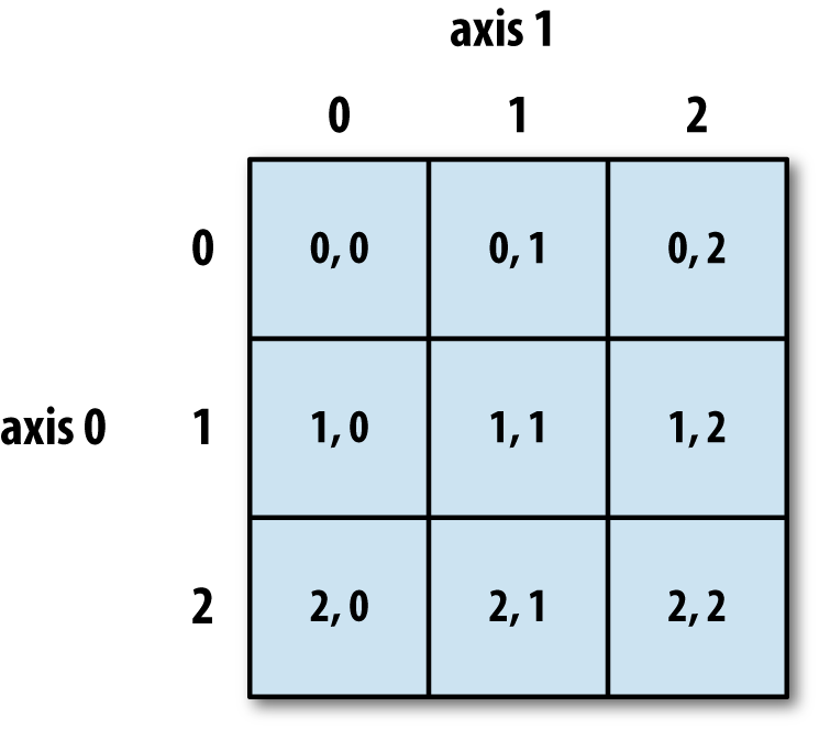
arr2d[0, 2]3A nice visual of a 2D array

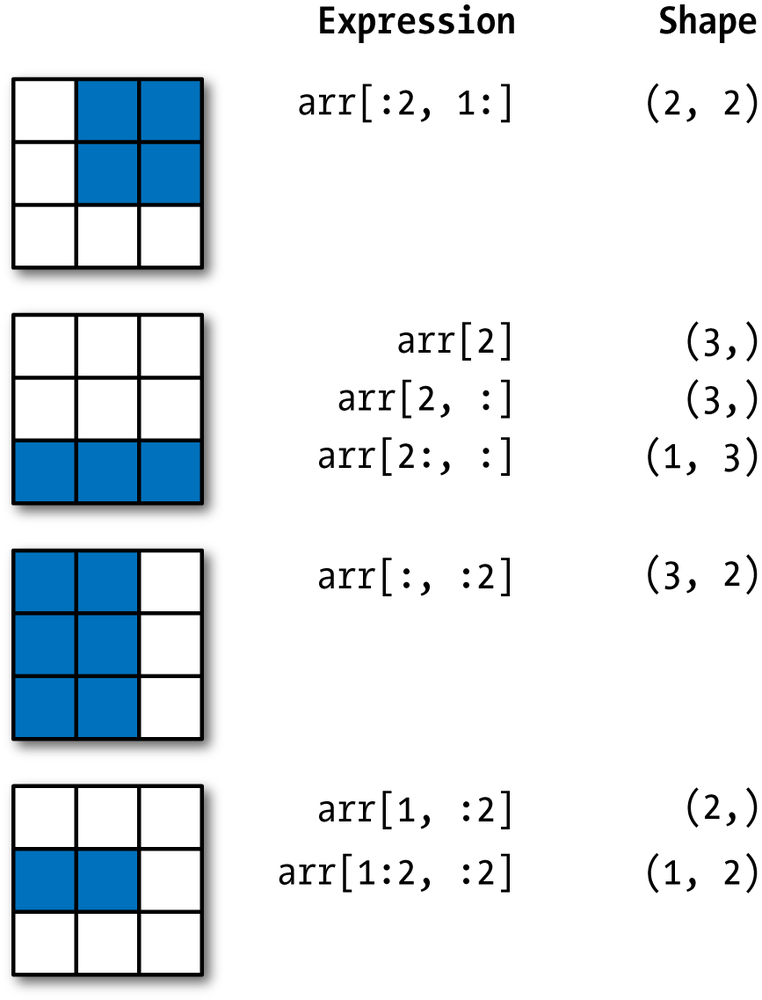
Two-Demensional Array Slicing

3D arrays
arr3d = np.array([[[1, 2, 3], [4, 5, 6]], [[7, 8, 9], [10, 11, 12]]])arr3d.shape(2, 2, 3)arr3darray([[[ 1, 2, 3],
[ 4, 5, 6]],
[[ 7, 8, 9],
[10, 11, 12]]])I find NumPy’s way of show the data a bit difficult to parse visually.
Here is a way to visualize 3 and higher dimensional data:
[ # AXIS 0                     AXIS 1 CONTAINS 2 ELEMENTS (arrays)
    [ # AXIS 1                 EACH MEMBER OF AXIS 2 CONTAINS 2 ELEMENTS (arrays)
        [1, 2, 3], # AXIS 2    EACH MEMBER OF AXIS 3 CONTAINS 3 ELEMENTS (integers)
        [4, 5, 6]  # AXIS 2
    ],
    [ # AXIS 1
        [7, 8, 9],
        [10, 11, 12]
    ]
]
Each axis is a level in the nested hierarchy, i.e. a tree or DAG (directed-acyclic graph).
- Each axis is a container.
- There is only one top container.
- Only the bottom containers have data.
Omit lower indices
In multidimensional arrays, if you omit later indices, the returned object will be a lower-dimensional ndarray consisting of all the data contained by the higher indexed dimension.
So in the 2 × 2 × 3 array arr3d:
arr3d[0] # The elements contained by the first rowarray([[1, 2, 3],
[4, 5, 6]])Saving data before modifying an array.
You can work with these lower dimensional arrays using views and copies.
old_values = arr3d[0].copy() # Make a copy
arr3d[0] = 42                # Use a view to alter the original
arr3d                        # See result
array([[[42, 42, 42],
[42, 42, 42]],
[[ 7, 8, 9],
[10, 11, 12]]])Putting the data back.
arr3d[0] = old_values
arr3d
array([[[ 1, 2, 3],
[ 4, 5, 6]],
[[ 7, 8, 9],
[10, 11, 12]]])Similarly, arr3d[1, 0] gives you all of the values whose indices start with (1, 0), forming a 1-dimensional array:
arr3d[1, 0]array([7, 8, 9])x = arr3d[1]
xarray([[ 7, 8, 9],
[10, 11, 12]])x[0]array([7, 8, 9])Indexing 2D arrays with slices
We demonstrate indexing in 2D arrays.
arrarray([ 0, 1, 2, 3, 4, 64, 64, 64, 8, 9])arr[1:6]array([ 1, 2, 3, 4, 64])arr2darray([[1, 2, 3],
[4, 5, 6],
[7, 8, 9]])arr2d[:2]array([[1, 2, 3],
[4, 5, 6]])arr2d[:2, 1:]array([[2, 3],
[5, 6]])arr2d[1, :2]array([4, 5])arr2d[:2, 2]array([3, 6])arr2d[:, :1]array([[1],
[4],
[7]])arr2d[:2, 1:] = 0
arr2darray([[1, 0, 0],
[4, 0, 0],
[7, 8, 9]])Boolean Indexing
This a crucial topic – it applies to Pandas and R.
You can pass a boolean representation of an array to the array indexer (i.e. the [] suffix) and it will return only those cells that are True.
Let’s assume that we have two related arrays: * names which holds the names associated with the data in each row, or observations, of a table. * data which holds the data associated with each feature of a table.
There are \(7\) observations and \(4\) features.
names = np.array(['Bob', 'Joe', 'Will', 'Bob', 'Will', 'Joe', 'Joe'])
names
array(['Bob', 'Joe', 'Will', 'Bob', 'Will', 'Joe', 'Joe'], dtype='<U4')data = np.random.randn(7, 4)
dataarray([[-0.30607318, -0.45423997, -0.91994934, -0.03050469],
[-0.4588956 , 0.92567072, -1.59370944, -0.71058406],
[ 1.77215664, -0.68150083, 1.95592254, 1.29936488],
[ 2.1290257 , 0.8816478 , 0.03409116, -2.25227674],
[ 0.49113167, -0.18440759, 0.32058921, 1.04615136],
[ 0.81208885, 1.62150232, -1.02330488, 0.67404131],
[-0.20037847, -0.51037469, 1.32144434, 1.56994506]])names.shape, data.shape((7,), (7, 4))A comparison operation for an array returns an array of booleans.
Let’s see which names are 'Bob':
names == 'Bob'array([ True, False, False, True, False, False, False])Now, this boolean expression can be passed to an array indexer to the data:
data[names == 'Bob']array([[-0.30607318, -0.45423997, -0.91994934, -0.03050469],
[ 2.1290257 , 0.8816478 , 0.03409116, -2.25227674]])Along the second axis, we can use a slice to select data.
data[names == 'Bob', 2:]array([[-0.91994934, -0.03050469],
[ 0.03409116, -2.25227674]])data[names == 'Bob', 3]array([-0.03050469, -2.25227674])If you know SQL, this is like the query:
SELECT col3, col4 FROM data WHERE name = 'Bob'Negation
Here are some examples of negated boolean operations being applied.
bix = names != 'Bob'
bix
array([False, True, True, False, True, True, True])data[bix]array([[-0.4588956 , 0.92567072, -1.59370944, -0.71058406],
[ 1.77215664, -0.68150083, 1.95592254, 1.29936488],
[ 0.49113167, -0.18440759, 0.32058921, 1.04615136],
[ 0.81208885, 1.62150232, -1.02330488, 0.67404131],
[-0.20037847, -0.51037469, 1.32144434, 1.56994506]])data[~bix] # Back to Bobarray([[-0.30607318, -0.45423997, -0.91994934, -0.03050469],
[ 2.1290257 , 0.8816478 , 0.03409116, -2.25227674]])data[~(names == 'Bob')]array([[-0.4588956 , 0.92567072, -1.59370944, -0.71058406],
[ 1.77215664, -0.68150083, 1.95592254, 1.29936488],
[ 0.49113167, -0.18440759, 0.32058921, 1.04615136],
[ 0.81208885, 1.62150232, -1.02330488, 0.67404131],
[-0.20037847, -0.51037469, 1.32144434, 1.56994506]])Note that we don’t use not but instead the tilde ~ sign to negate (flip) a value.
Nor do we use and and or; instead we use & and |.
Also, expressions join by these operators need to be in parentheses.
mask = (names == 'Bob') | (names == 'Will')
mask
data[mask]
array([[-0.30607318, -0.45423997, -0.91994934, -0.03050469],
[ 1.77215664, -0.68150083, 1.95592254, 1.29936488],
[ 2.1290257 , 0.8816478 , 0.03409116, -2.25227674],
[ 0.49113167, -0.18440759, 0.32058921, 1.04615136]])data[data < 0] = 0
dataarray([[0. , 0. , 0. , 0. ],
[0. , 0.92567072, 0. , 0. ],
[1.77215664, 0. , 1.95592254, 1.29936488],
[2.1290257 , 0.8816478 , 0.03409116, 0. ],
[0.49113167, 0. , 0.32058921, 1.04615136],
[0.81208885, 1.62150232, 0. , 0.67404131],
[0. , 0. , 1.32144434, 1.56994506]])data[names != 'Joe'] = 7
dataarray([[7. , 7. , 7. , 7. ],
[0. , 0.92567072, 0. , 0. ],
[7. , 7. , 7. , 7. ],
[7. , 7. , 7. , 7. ],
[7. , 7. , 7. , 7. ],
[0.81208885, 1.62150232, 0. , 0.67404131],
[0. , 0. , 1.32144434, 1.56994506]])Fancy Indexing
In so-call fancy indexing, we use array index numbers to access data.
This can be used to sub-select and re-order data from an array.
We pass a list of item numbers, instead of an integer or integer range with :, to the indexer.
arr = np.empty((8, 4))
for i in range(8):
    arr[i] = i
arr
array([[0., 0., 0., 0.],
[1., 1., 1., 1.],
[2., 2., 2., 2.],
[3., 3., 3., 3.],
[4., 4., 4., 4.],
[5., 5., 5., 5.],
[6., 6., 6., 6.],
[7., 7., 7., 7.]])The following says Select rows 4, 3, 0, and 6, in that order.
arr[[4, 3, 0, 6]]array([[4., 4., 4., 4.],
[3., 3., 3., 3.],
[0., 0., 0., 0.],
[6., 6., 6., 6.]])And we can go backwards.
arr[[-3, -5, -7]]array([[5., 5., 5., 5.],
[3., 3., 3., 3.],
[1., 1., 1., 1.]])We can use lists to perform some complex indexing.
arr = np.arange(32).reshape((8, 4))
arr
array([[ 0, 1, 2, 3],
[ 4, 5, 6, 7],
[ 8, 9, 10, 11],
[12, 13, 14, 15],
[16, 17, 18, 19],
[20, 21, 22, 23],
[24, 25, 26, 27],
[28, 29, 30, 31]])arr[[1, 5, 7, 2], [0, 3, 1, 2]] # Grab rows, then select columns from each rowarray([ 4, 23, 29, 10])arr[[1, 5, 7, 2]][:, [0, 3, 1, 2]] # Grab rows, then reorder columns array([[ 4, 7, 5, 6],
[20, 23, 21, 22],
[28, 31, 29, 30],
[ 8, 11, 9, 10]])Transposing Arrays and Swapping Axes
Transposing is a special form of reshaping which similarly returns a view on the underlying data without copying anything.
Arrays have the transpose method and also the special T attribute:
arr = np.arange(15).reshape((3, 5))
arr
array([[ 0, 1, 2, 3, 4],
[ 5, 6, 7, 8, 9],
[10, 11, 12, 13, 14]])arr.Tarray([[ 0, 5, 10],
[ 1, 6, 11],
[ 2, 7, 12],
[ 3, 8, 13],
[ 4, 9, 14]])Transposing is often used when computing the dot product between two arrays.
Here’s an example.
arr = np.random.randn(6, 3)
arr
array([[-0.71192017, 1.12793945, 0.00398408],
[-0.33313537, -0.05308562, 0.73532491],
[-1.34038679, -0.6211279 , -1.72999099],
[ 0.41464889, 0.31148611, -1.61275124],
[ 0.34175606, -0.23790281, -0.37332351],
[ 1.01792075, -0.5389869 , 1.46791149]])np.dot(arr.T, arr)array([[ 3.73933981, -0.45355983, 2.76896447],
[-0.45355983, 2.10499356, -0.16471567],
[ 2.76896447, -0.16471567, 8.42868857]])For higher dimensional arrays, transpose will accept a tuple of axis numbers to permute the axes.
Warning – this can get confusing to conceptualize and visualize!
arr = np.arange(16).reshape((2, 2, 4))
arr
array([[[ 0, 1, 2, 3],
[ 4, 5, 6, 7]],
[[ 8, 9, 10, 11],
[12, 13, 14, 15]]])arr.transpose((1, 0, 2))array([[[ 0, 1, 2, 3],
[ 8, 9, 10, 11]],
[[ 4, 5, 6, 7],
[12, 13, 14, 15]]])Simple transposing with .T is just a special case of swapping axes. ndarray has the method swapaxes which takes a pair of axis numbers:
arrarray([[[ 0, 1, 2, 3],
[ 4, 5, 6, 7]],
[[ 8, 9, 10, 11],
[12, 13, 14, 15]]])arr.swapaxes(1, 2)array([[[ 0, 4],
[ 1, 5],
[ 2, 6],
[ 3, 7]],
[[ 8, 12],
[ 9, 13],
[10, 14],
[11, 15]]])Universal Functions
A universal function, or ufunc, is a function that performs elementwise operations on data in ndarrays. You can think of them as fast vectorized wrappers for simple functions that take one or more scalar values and produce one or more scalar results.
Many ufuncs are simple elementwise transformations, like sqrt or exp:
arr = np.arange(10)
arr
array([0, 1, 2, 3, 4, 5, 6, 7, 8, 9])np.sqrt(arr)array([0. , 1. , 1.41421356, 1.73205081, 2. ,
2.23606798, 2.44948974, 2.64575131, 2.82842712, 3. ])np.exp(arr)array([1.00000000e+00, 2.71828183e+00, 7.38905610e+00, 2.00855369e+01,
5.45981500e+01, 1.48413159e+02, 4.03428793e+02, 1.09663316e+03,
2.98095799e+03, 8.10308393e+03])x = np.random.randn(8)
xarray([-0.81849005, -0.03252903, -0.78588415, -0.75569246, 0.28011989,
-0.07210453, -1.33721432, 0.57725791])y = np.random.randn(8)
yarray([ 0.45964976, 0.2479025 , 0.655078 , -0.16776598, 1.81773551,
-0.568098 , 0.01841105, 0.64186879])np.maximum(x, y)array([ 0.45964976, 0.2479025 , 0.655078 , -0.16776598, 1.81773551,
-0.07210453, 0.01841105, 0.64186879])arr = np.random.randn(7) * 5
arrarray([-1.07243891, 0.06744552, -5.00862819, -2.07837886, 3.17212965,
5.69620434, -1.53635927])remainder, whole_part = np.modf(arr)
remainderarray([-0.07243891, 0.06744552, -0.00862819, -0.07837886, 0.17212965,
0.69620434, -0.53635927])whole_partarray([-1., 0., -5., -2., 3., 5., -1.])arrarray([-1.07243891, 0.06744552, -5.00862819, -2.07837886, 3.17212965,
5.69620434, -1.53635927])np.sqrt(arr)/var/folders/14/rnyfspnx2q131jp_752t9fc80000gn/T/ipykernel_25317/983116409.py:2: RuntimeWarning: invalid value encountered in sqrt
np.sqrt(arr)array([ nan, 0.25970275, nan, nan, 1.78104735,
2.38667223, nan])np.sqrt(arr, arr)/var/folders/14/rnyfspnx2q131jp_752t9fc80000gn/T/ipykernel_25317/1230165595.py:2: RuntimeWarning: invalid value encountered in sqrt
np.sqrt(arr, arr)array([ nan, 0.25970275, nan, nan, 1.78104735,
2.38667223, nan])arrarray([ nan, 0.25970275, nan, nan, 1.78104735,
2.38667223, nan])nan is a special value in NumPy.