NB: Loose Ends

options(warn = -1) # Turn off warnings

library(vctrs) # This fixes the vec_as_location() problem
library(tidyverse)

qplot

qplot creates quick and simple plots that use all of the ggplot2 defaults.

It let’s you define a plot in a single call that gives a set of aesthetics and a data set.

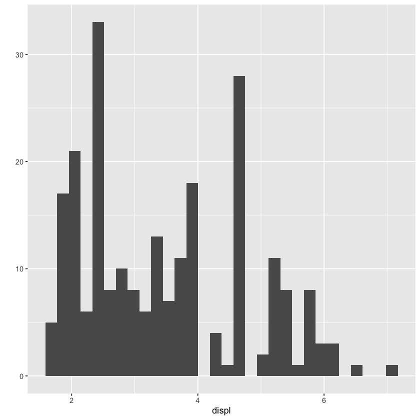
It infers a geom from your data and mappings if you don’t supply onw. Recall this is how plot worked.

plot(select(iris, -Species))

# qplot(select(iris, -Species))

qplot(displ, hwy, data = mpg)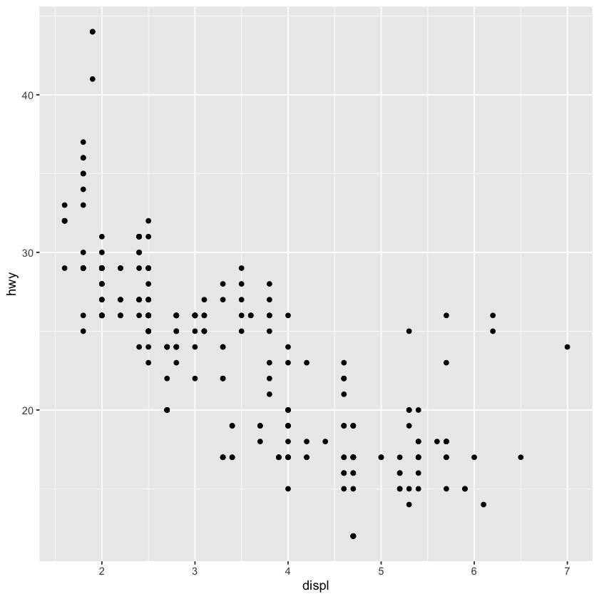

qplot(displ, hwy, color=class, data = mpg)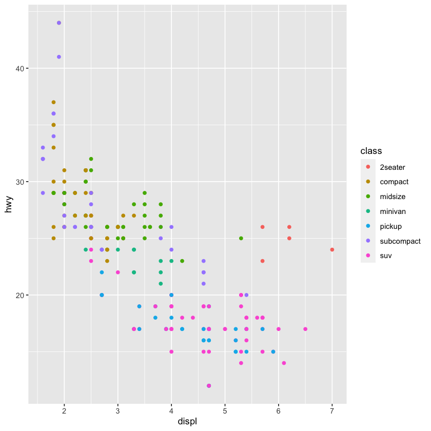

qplot(displ, data = mpg)

`stat_bin()` using `bins = 30`. Pick better value with `binwidth`.

qplot(displ, data = mpg, geom = c('bar'))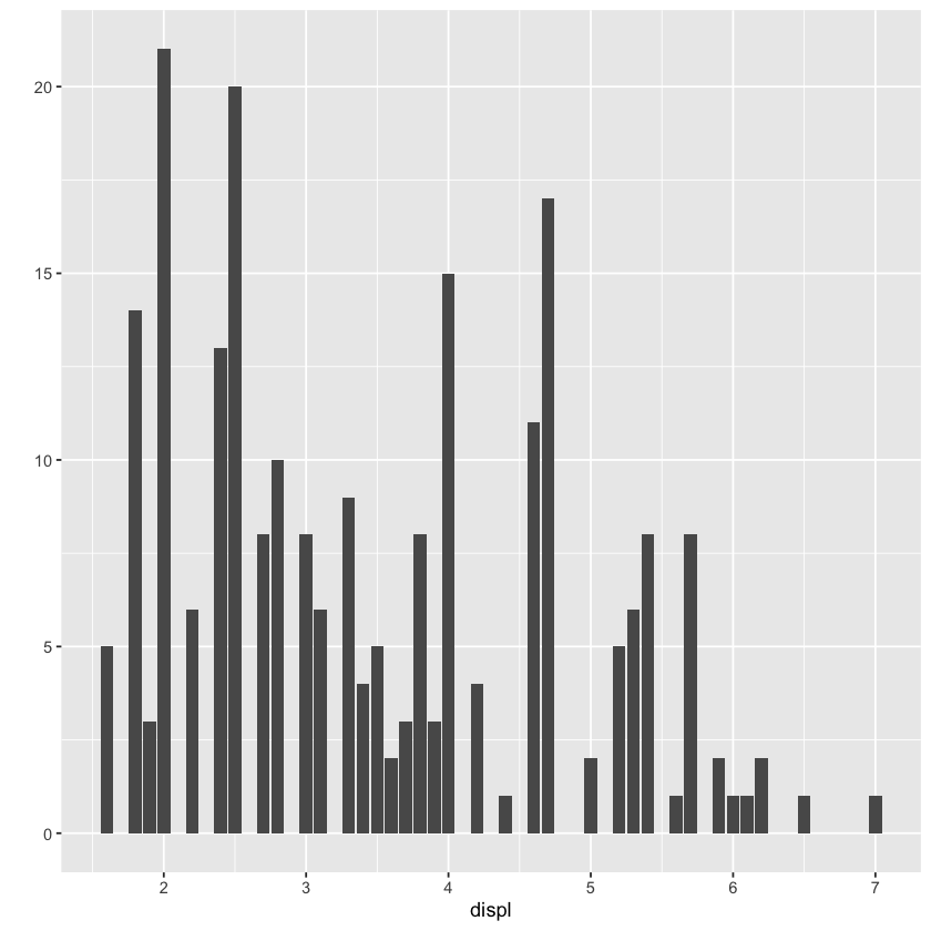

Gotchas

Oddly, data is not the first argument, so it won’t work with %>%.

This will fail:

# mpg %>% qplot(displ, hwy)

Also, data has to be called by key, e.g. data = mpg.

This will fail, too:

# qplot(displ, hwy, mpg)

Here’s a nice guide in PDF form: Getting started with qplot

GGPlot in Python

There are pygg plotnine and

Hard to replicate R syntax in Python.

But why should it? Should just implement to pattern Pythonically.

See example in M14-00a-Plotnine.ipynb.

Plotly in R

install.packages("plotly")

  There is a binary version available but the source version is later:
       binary source needs_compilation
plotly 4.10.0 4.10.2             FALSE

installing the source package ‘plotly’

library(plotly)

Attaching package: ‘plotly’


The following object is masked from ‘package:ggplot2’:

    last_plot


The following object is masked from ‘package:stats’:

    filter


The following object is masked from ‘package:graphics’:

    layout

Types of plots

'bar', 'barpolar', 'box', 'candlestick', 'carpet', 'choropleth', 'choroplethmapbox', 'cone', 'contour', 'contourcarpet', 'densitymapbox', 'funnel', 'funnelarea', 'heatmap', 'heatmapgl', 'histogram', 'histogram2d', 'histogram2dcontour', 'icicle', 'image', 'indicator', 'isosurface', 'mesh3d', 'ohlc', 'parcats', 'parcoords', 'pie', 'pointcloud', 'sankey', 'scatter', 'scatter3d', 'scattercarpet', 'scattergeo', 'scattergl', 'scattermapbox', 'scatterpolar', 'scatterpolargl', 'scatterternary', 'splom', 'streamtube', 'sunburst', 'surface', 'table', 'treemap', 'violin', 'volume', 'waterfall'

head(mpg)

A tibble: 6 × 11

manufacturer	model	displ	year	cyl	trans	drv	cty	hwy	fl	class
<chr>	<chr>	<dbl>	<int>	<int>	<chr>	<chr>	<int>	<int>	<chr>	<chr>
audi	a4	1.8	1999	4	auto(l5)	f	18	29	p	compact
audi	a4	1.8	1999	4	manual(m5)	f	21	29	p	compact
audi	a4	2.0	2008	4	manual(m6)	f	20	31	p	compact
audi	a4	2.0	2008	4	auto(av)	f	21	30	p	compact
audi	a4	2.8	1999	6	auto(l5)	f	16	26	p	compact
audi	a4	2.8	1999	6	manual(m5)	f	18	26	p	compact

fig1 <- mpg %>%
    plot_ly(
        x         = ~hwy, 
        y         = ~cty, 
        size      = ~displ, 
        type      = 'scatter', 
        color     = ~class,
        mode      = "markers",
        hovertext = ~manufacturer,
        height    = 500, width = 750)

fig1

fig2 <- iris %>%
    plot_ly(
        x         = ~Petal.Length, 
        y         = ~Petal.Width, 
        size      = ~Sepal.Length, 
        color     = ~Sepal.Width,
        symbol    = ~Species,
        type      = "scatter", 
        mode      = "markers",
        height    = 500, width = 750)

fig2

# ?plot_ly

GGPlotly

Best of both worlds?

With ggplotly() by Plotly, you can convert your ggplot2 figures into interactive ones powered by plotly.js, ready for embedding into Dash applications.

If you call ggplotly() with no argument, it will display your last ggplot as a plotly plot.

Pretty cool.

You also pass it a plot that was assigned to a variable.

In both cases, you can then add ploty features to your graph.

df = data.frame(
    x = 1:10,
    y = 1:100:10
)

df %>% ggplot() + 
    aes(x, y) +
    geom_line()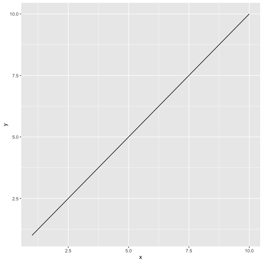

ggplotly()

ggplotly(height=400, width=400)

p = df %>% ggplot() + 
    aes(x, y) +
    geom_line()

ggplotly(p)

>>> Learn more.

Using :: in R

When you load libraries in R that have the same function names, R resolves this by picking a default, and then letting you access the others using :: operator to specify the library from which the method comes.

The rule is that the package loaded last will hide, or mask, the function from earlier packages.

If you want to have a certain function be the default, make sure you load it last.

For example, when we load tidyverse, we get this message:

✖ dplyr::filter() masks stats::filter()
✖ dplyr::lag()    masks stats::lag()

This means that dplyr overrides the filter() and lag() methods associated with the stats library.

Similarly, when you load plotly, you’ll see this:

Attaching package: ‘plotly’

The following object is masked from ‘package:ggplot2’:

    last_plot

The following object is masked from ‘package:stats’:

    filter

The following object is masked from ‘package:graphics’:

    layout

One thing I have noticed is that even though the last library masks the other functions, the help operator ?<objectname> does not follow this.

Also, in this script, note that dplyr::filter is the default, even though plotly::filter loaded after dplyr. This is because Plotly’ filter function is not used in the normal way; it appears in the context of the transforms argument to plot_ly(). No need to get into this now, but just know that that’s why it does not mask dplyr.

Examples

Here, we call filter by itself and it uses the one from dplyr.

head(filter(mpg, hwy > 0))

But if we ask for help, we’ll get the original stats version.

# ?filter

And if we ask for help about Plotly’s version, we see this:

# ?plotly