NB: NumPy Indexing

Programming for Data Science

Indexing

Now that we have learned about the basic structure of NumPy’s multidimensional arrays, let’s look at how to access and extract subsets of data from them.

Here is a \(2\)-D array, or matrix, initialized from a list of lists.

import numpy as np
arr2d = np.array([[1, 2, 3], [4, 5, 6], [7, 8, 9]])
arr2d

array([[1, 2, 3],
       [4, 5, 6],
       [7, 8, 9]])

If we wanted to get the third row of the matrix, we can do this:

arr2d[2]

array([7, 8, 9])

This is called indexing, and it is similar to what we learned about accessing data from lists, tuples, and other sequences in basic Python.

Indexing into an axis produces lower-order arrays.

Here we returned a \(1\)-D array from a \(2\)-D one.

Simplified Notation

Let’s say we wanted to extract a single scalar from the matrix.

We could do this to get the third cell from the first row:

arr2d[0][2]

3

NumPy offers a simpler way to index mulitple axes.

Instead of x[a][b][c] you can write x[a, b, c].

Think of this as similar to how NumPy represents shape as a tuple.

Each element of the array has an index tuple, which is really a coordinate.

So, in this case, we could do this:

arr2d[0, 2]

3

Or, thinking of the cell as a point in \(2\)-D space:

my_cell_coord = (0,2)
arr2d[my_cell_coord]

3

Let’s look at a cube:

arr3d = np.array([[[1, 2, 3], [4, 5, 6]], [[7, 8, 9], [10, 11, 12]]])

arr3d

array([[[ 1,  2,  3],
        [ 4,  5,  6]],

       [[ 7,  8,  9],
        [10, 11, 12]]])

This is how we could access the (1,0,2) coordinate:

arr3d[1, 0, 2]

9

Visualizing Array Structure

Here is a way to help you visualize 3 and higher dimensional data:

[ # AXIS 0                       AXIS 0: CONTAINS 2 matrices
    [ # AXIS 1                   AXIS 1: EACH MEMBER CONTAINS 2 vectors
        [1, 2, 3],   # AXIS 2    AXIS 2: EACH MEMBER CONTAINS 3 scalars
        [4, 5, 6]    # AXIS 2
    ],  
    [ # AXIS 1
        [7, 8, 9],   # AXIS 2
        [10, 11, 12] # AXIS 2
    ]
]

Each axis is a level in the nested hierarchy, like a tree or DAG (directed-acyclic graph).

Each axis is a container of a lower-order array — the cube contains matrices with contain vectors which contain scalars.

There is only one top container.

Only the bottom containers have scalar data — the numbers.

So, if you omit later indices of an array, the returned object will be a lower-dimensional array consisting of all the data contained by the higher indexed dimension.

So, with arr3d, selecting an element from the first axis, we get a matrix from a cube:

arr3d[0]

array([[1, 2, 3],
       [4, 5, 6]])

Similarly, arr3d[1, 0] gives you all of the values whose indices start with (1, 0), forming a 1-dimensional array:

arr3d[1, 0]

array([7, 8, 9])

Slicing

Slicing refers to selecting subsets of arrays.

It is like selecting in SQL — you ask for parts of an array.

Let’s look at some examples.

Here is a vector.

arr1d = np.random.randint(1, 100, 10)
arr1d

array([76, 46, 76, 64, 37, 11, 43, 75, 42, 71])

By using the colon : notation, we can select a vector with the second through the fifth elements.

arr1d[1:6]

array([46, 76, 64, 37, 11])

Here is a matrix.

arr2d

array([[1, 2, 3],
       [4, 5, 6],
       [7, 8, 9]])

By omitting the first number, NumPy defaults to the beginning \(0\).

This returns the first two elements of the top level, which means two rows:

arr2d[:2]

array([[1, 2, 3],
       [4, 5, 6]])

Here we grab the first two rows, and then, for each row, we omit the first element:

arr2d[:2, 1:]

array([[2, 3],
       [5, 6]])

And here are some more examples of slicing into a matrix:

arr2d[1, :2]

array([4, 5])

arr2d[:2, 2]

array([3, 6])

arr2d[:, :1]

array([[1],
       [4],
       [7]])

Shapes

Recall that there is a difference between a \(1\)-dimensional array and an \(2\)-dimensional array with one row or column.

This comes up again in slices.

Consider the following examples.

Here we compare a slice that extracts a single row, and a simple index that extracts a the same row.

arr2d[0:1], arr2d[0]

(array([[1, 2, 3]]), array([1, 2, 3]))

arr2d[0:1].shape, arr2d[0].shape

((1, 3), (3,))

Note the difference in shape.

A range, even of length \(1\), returns a slice, which is always a sequence.

In this case, the range selects a 1-element sequence of vectors, while the simple index selects the element itself.

Let’s look at a higher-order array.

In the first axis selector, we use a scalar in one case and a slice in the other.

arr3d[1, :], arr3d[1:, :]

(array([[ 7,  8,  9],
        [10, 11, 12]]),
 array([[[ 7,  8,  9],
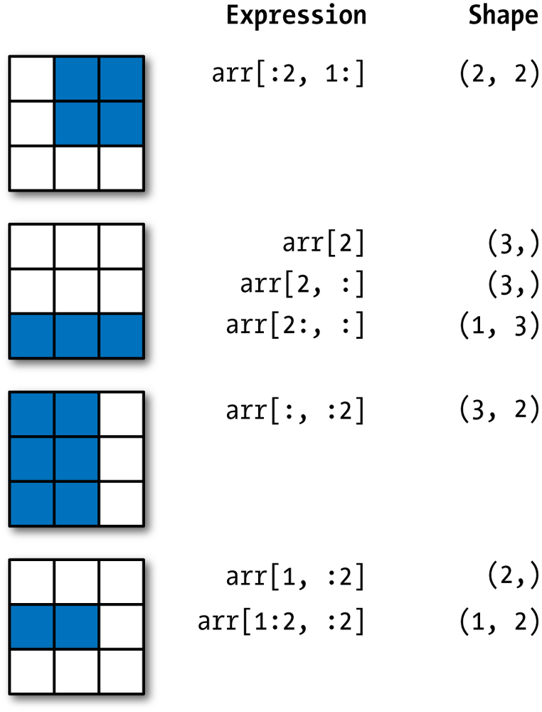
         [10, 11, 12]]]))

arr3d[1, :].shape, arr3d[1:, :].shape

((2, 3), (1, 2, 3))

Another Visual

Here is a nice visualization of how slicing works, taken from McKinney 2017, Chapter 4.

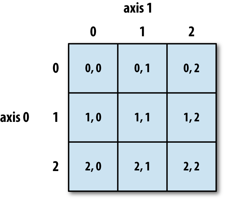
Consider the following \(2\)-D array. Each cell is labeled by its address.

Here are some slices and their return values.

Altering Values

Slices can be used to extract subsets of data, but we may also use them to alter subsets as well.

Here we set all the values of a slice to \(0\).

arr2d[:2, 1:] = 0
arr2d

array([[1, 0, 0],
       [4, 0, 0],
       [7, 8, 9]])

Views

It is crucial to understand when altering the results of a slicing or indexing operation , NumPy returns views to the source object, not copies of it.

That is the two variables both point to the same object.

This means if we assign a slice to a variable and alter the new variable, we also alter the original!

Let’s illustrate this with an example. See what happens when we change a view.

Here we assign a slice to a variable.

arr_slice = arr2d[2:3]
arr_slice

array([[7, 8, 9]])

Then we alter the data in the variable.

arr_slice[0,2] = 12345

But notice how it changes our original:

arr2d

array([[    1,     0,     0],
       [    4,     0,     0],
       [    7,     8, 12345]])

Here’s another example, to reinforce the point.

arr_slice[:] = 64

arr_slice

array([[64, 64, 64]])

arr2d

array([[ 1,  0,  0],
       [ 4,  0,  0],
       [64, 64, 64]])

Copies

NumPy defaults to views rather than copies because copies are expensive.

This is because NumPy is designed with large data use cases in mind.

If you want a copy of a slice of an array instead of a view, use .copy().

Here’s an example:

arr_slice_copy = arr2d[2:3].copy()
arr_slice_copy

array([[64, 64, 64]])

arr_slice_copy[:] = 99
arr_slice_copy

array([[99, 99, 99]])

Note how the original array is unchanged:

arr2d

array([[ 1,  0,  0],
       [ 4,  0,  0],
       [64, 64, 64]])

One pattern to follow is to save data before modifying an array.

arr3d[0]

array([[1, 2, 3],
       [4, 5, 6]])

saved_data = arr3d[0].copy()
arr3d[0] = 42
arr3d

array([[[42, 42, 42],
        [42, 42, 42]],

       [[ 7,  8,  9],
        [10, 11, 12]]])

Putting the data back.

arr3d[0] = saved_data
arr3d

array([[[ 1,  2,  3],
        [ 4,  5,  6]],

       [[ 7,  8,  9],
        [10, 11, 12]]])

Fancy Indexing

In addition to passing integers and slices to the array indexer, we can pass lists of array index numbers for each axis.

This is called fancy indexing.

This can be used to both sub-select and re-order data from an array.

Here’s an example.

We create an empty \(8 \times 4\) array and then immediately re-populate it.

arr = np.empty((8, 4))
for i in range(arr.shape[0]):
    arr[i] = i
arr

array([[0., 0., 0., 0.],
       [1., 1., 1., 1.],
       [2., 2., 2., 2.],
       [3., 3., 3., 3.],
       [4., 4., 4., 4.],
       [5., 5., 5., 5.],
       [6., 6., 6., 6.],
       [7., 7., 7., 7.]])

The following fancy index selects rows 4, 3, 0, and 6, in that order:

arr[[4, 3, 0, 6]]

array([[4., 4., 4., 4.],
       [3., 3., 3., 3.],
       [0., 0., 0., 0.],
       [6., 6., 6., 6.]])

We can also go backwards, just as we can index elements of a list.

arr[[-3, -5, -7]]

array([[5., 5., 5., 5.],
       [3., 3., 3., 3.],
       [1., 1., 1., 1.]])

We can also use lists to perform some complex indexing.

arr = np.arange(32).reshape((8, 4))
arr

array([[ 0,  1,  2,  3],
       [ 4,  5,  6,  7],
       [ 8,  9, 10, 11],
       [12, 13, 14, 15],
       [16, 17, 18, 19],
       [20, 21, 22, 23],
       [24, 25, 26, 27],
       [28, 29, 30, 31]])

Here we grab rows, then select columns from each row.

arr[[1, 5, 7, 2], [0, 3, 1, 2]]

array([ 4, 23, 29, 10])

And here we grab some rows in a particular order, then re-order the columns.

arr[[1, 5, 7, 2]][:, [0, 3, 1, 2]] 

array([[ 4,  7,  5,  6],
       [20, 23, 21, 22],
       [28, 31, 29, 30],
       [ 8, 11,  9, 10]])

Something to be Aware of

There is a difference between doing this arr[1:, :2] …

and doing this arr[1:][:2].

The first case operates on both axes simultaneousy, slicing both rows and columns.

The second case operates on the axes sequentially, slicing rows then rows again.

This may be confusing, since the two notations are the same when we are not using slices.

Here is an example.

foo = np.random.randn(3,5)

foo

array([[ 0.88095771,  0.17701757,  0.69125263,  0.67894113,  0.1763698 ],
       [ 0.17465033, -0.25317231,  0.45904164,  0.21024919,  1.11688081],
       [-0.52672375, -0.09234619, -0.46120961, -0.1940446 , -0.28382698]])

Now, this slices rows and columns:

foo[1:, :2]

array([[ 0.17465033, -0.25317231],
       [-0.52672375, -0.09234619]])

And this slices rows, then rows again on the result:

foo[1:][:2]

array([[ 0.17465033, -0.25317231,  0.45904164,  0.21024919,  1.11688081],
       [-0.52672375, -0.09234619, -0.46120961, -0.1940446 , -0.28382698]])