NB: GGPlot in Python with Plotnine

Programming for Data Science

GGPlot in Python

There are two ports of GGPlot2 to Python: pygg and plotnine.

The first seems to have stopped development and is much less used.

Let’s look at Plotnine.

# ! conda install -c conda-forge plotnine -y

from plotnine import *
from plotnine.data import mpg

Our old friend, mpg in Python:

mpg

	manufacturer	model	displ	year	cyl	trans	drv	cty	hwy	fl	class
0	audi	a4	1.8	1999	4	auto(l5)	f	18	29	p	compact
1	audi	a4	1.8	1999	4	manual(m5)	f	21	29	p	compact
2	audi	a4	2.0	2008	4	manual(m6)	f	20	31	p	compact
3	audi	a4	2.0	2008	4	auto(av)	f	21	30	p	compact
4	audi	a4	2.8	1999	6	auto(l5)	f	16	26	p	compact
...	...	...	...	...	...	...	...	...	...	...	...
229	volkswagen	passat	2.0	2008	4	auto(s6)	f	19	28	p	midsize
230	volkswagen	passat	2.0	2008	4	manual(m6)	f	21	29	p	midsize
231	volkswagen	passat	2.8	1999	6	auto(l5)	f	16	26	p	midsize
232	volkswagen	passat	2.8	1999	6	manual(m5)	f	18	26	p	midsize
233	volkswagen	passat	3.6	2008	6	auto(s6)	f	17	26	p	midsize

234 rows × 11 columns

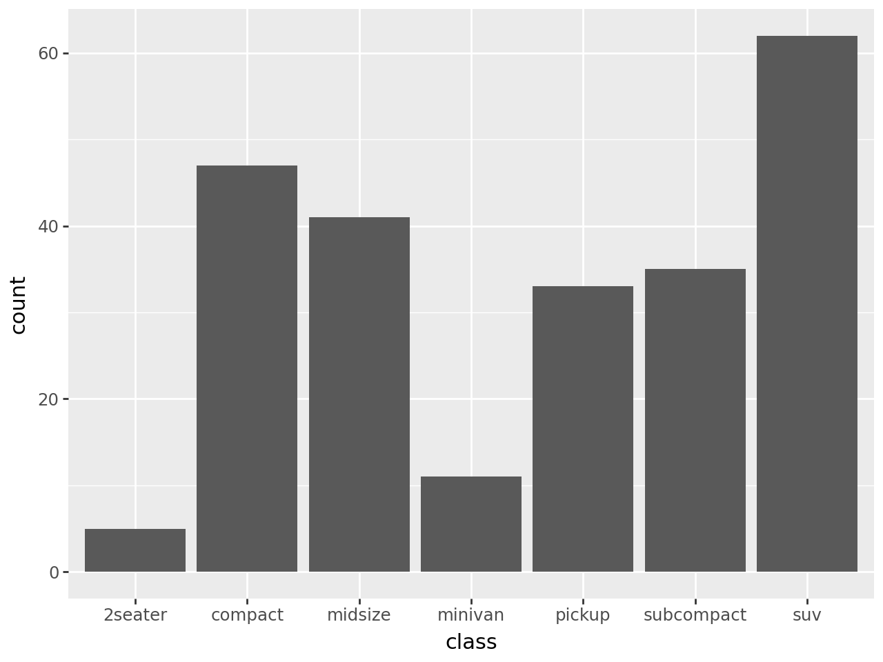
A Simple Bar Chart

(ggplot(mpg)            # defining what data to use
    + aes(x='class')    # defining what variable to use
    + geom_bar(size=20) # defining the type of plot to use
)

Notice that aes() is not a helper function (a function in the argument space).

Also, R dots become _ in the argument names.

Note that we don’t have to use the syntax above, which groups the functions in a single expression with (...).

We can do this:

ggplot(mpg) + aes(x='class') + geom_bar(size=20)

Or this:

ggplot(mpg) + \
    aes(x='class') + \
    geom_bar(size=20)

Note that none of these are like R due to differing white space rules.

Aesthetics

Plotnine supports using color and size on which to map features with aes().

ggplot(mpg) + \
    aes(x = 'drv', y = 'cty', color = 'class', size='cyl') + \
    geom_point()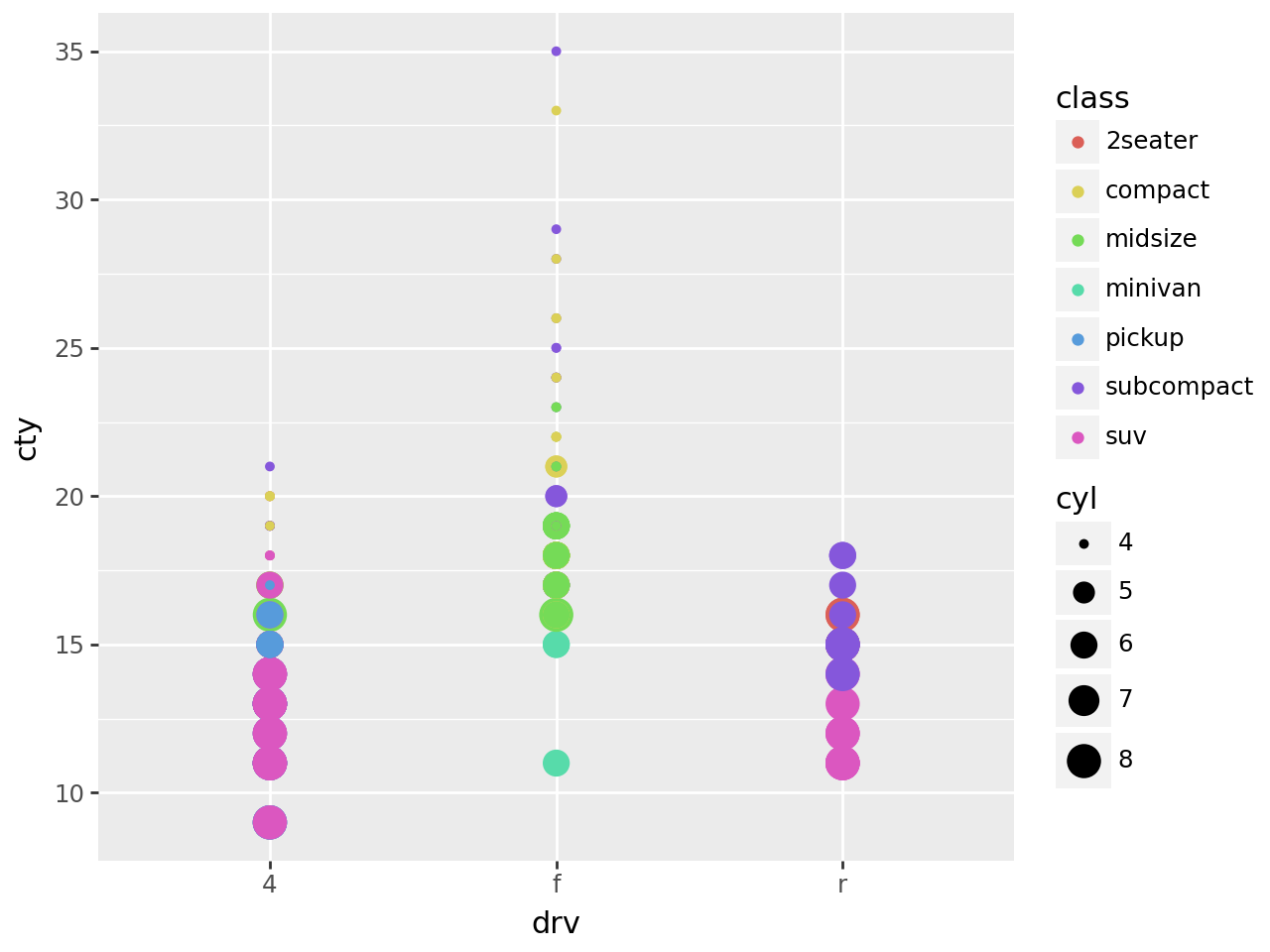

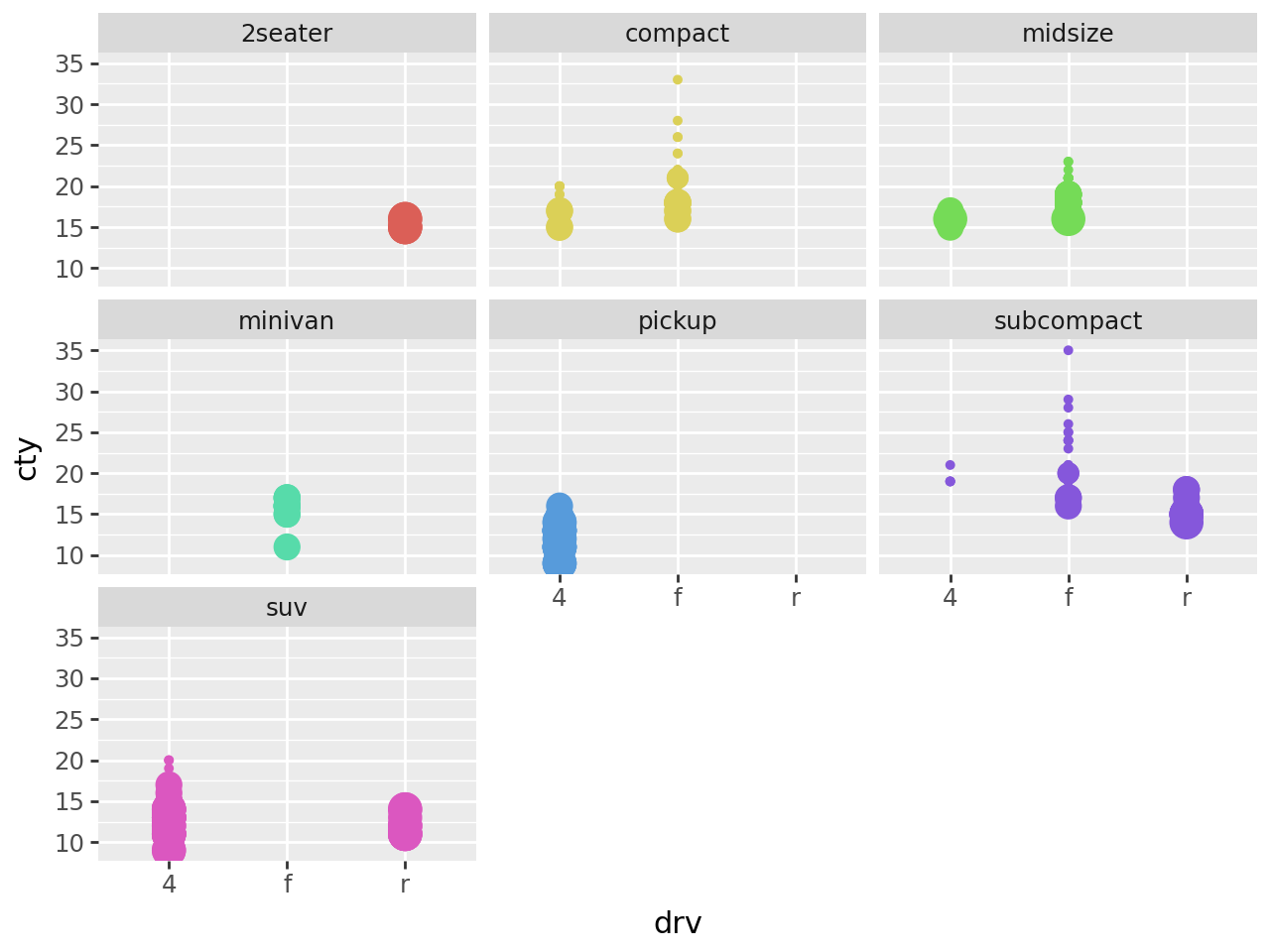
Facets

You can also create facets with facet_wrap().

(ggplot(mpg)         
 + aes(x='drv', y='cty', color='class', size='cyl')
 + geom_point()
 + facet_wrap('class')
 + theme(legend_position = "none")
)