NB: R Data Frames

Programming for Data Science

Data Frames

A data frame is used for storing data tables.

It is essentially a list of vectors of equal length.

For example, the following variable df is a data frame containing three vectors n, s, b.

n <- c(2, 3, 5) 
s <- c("aa", "bb", "cc") 
b <- c(TRUE, FALSE, TRUE) 
df <- data.frame(n, s, b)
df

A data.frame: 3 × 3

n	s	b
<dbl>	<chr>	<lgl>
2	aa	TRUE
3	bb	FALSE
5	cc	TRUE

Notice that data frames are built column-wise.

When displayed in certain environemnts, the top line of the data frame is the header and it contains the column names.

The data type is listed below the column name.

Each horizontal line afterward denotes a data row, which may begin with the name of the row, and then followed by the actual data.

Each data member of a row is called a cell.

Note that on Jupyter, if we print a data frame, we get this:

print(df)

  n  s     b
1 2 aa  TRUE
2 3 bb FALSE
3 5 cc  TRUE

Built-in Data Frames

To learn more about data frames in R, let’s look at some built in data.

R comes with many built-in data sets to get you started.

These do not need to be imported.

Here is the mtcars data frame.

mtcars

A data.frame: 32 × 11

	mpg	cyl	disp	hp	drat	wt	qsec	vs	am	gear	carb
	<dbl>	<dbl>	<dbl>	<dbl>	<dbl>	<dbl>	<dbl>	<dbl>	<dbl>	<dbl>	<dbl>
Mazda RX4	21.0	6	160.0	110	3.90	2.620	16.46	0	1	4	4
Mazda RX4 Wag	21.0	6	160.0	110	3.90	2.875	17.02	0	1	4	4
Datsun 710	22.8	4	108.0	93	3.85	2.320	18.61	1	1	4	1
Hornet 4 Drive	21.4	6	258.0	110	3.08	3.215	19.44	1	0	3	1
Hornet Sportabout	18.7	8	360.0	175	3.15	3.440	17.02	0	0	3	2
Valiant	18.1	6	225.0	105	2.76	3.460	20.22	1	0	3	1
Duster 360	14.3	8	360.0	245	3.21	3.570	15.84	0	0	3	4
Merc 240D	24.4	4	146.7	62	3.69	3.190	20.00	1	0	4	2
Merc 230	22.8	4	140.8	95	3.92	3.150	22.90	1	0	4	2
Merc 280	19.2	6	167.6	123	3.92	3.440	18.30	1	0	4	4
Merc 280C	17.8	6	167.6	123	3.92	3.440	18.90	1	0	4	4
Merc 450SE	16.4	8	275.8	180	3.07	4.070	17.40	0	0	3	3
Merc 450SL	17.3	8	275.8	180	3.07	3.730	17.60	0	0	3	3
Merc 450SLC	15.2	8	275.8	180	3.07	3.780	18.00	0	0	3	3
Cadillac Fleetwood	10.4	8	472.0	205	2.93	5.250	17.98	0	0	3	4
Lincoln Continental	10.4	8	460.0	215	3.00	5.424	17.82	0	0	3	4
Chrysler Imperial	14.7	8	440.0	230	3.23	5.345	17.42	0	0	3	4
Fiat 128	32.4	4	78.7	66	4.08	2.200	19.47	1	1	4	1
Honda Civic	30.4	4	75.7	52	4.93	1.615	18.52	1	1	4	2
Toyota Corolla	33.9	4	71.1	65	4.22	1.835	19.90	1	1	4	1
Toyota Corona	21.5	4	120.1	97	3.70	2.465	20.01	1	0	3	1
Dodge Challenger	15.5	8	318.0	150	2.76	3.520	16.87	0	0	3	2
AMC Javelin	15.2	8	304.0	150	3.15	3.435	17.30	0	0	3	2
Camaro Z28	13.3	8	350.0	245	3.73	3.840	15.41	0	0	3	4
Pontiac Firebird	19.2	8	400.0	175	3.08	3.845	17.05	0	0	3	2
Fiat X1-9	27.3	4	79.0	66	4.08	1.935	18.90	1	1	4	1
Porsche 914-2	26.0	4	120.3	91	4.43	2.140	16.70	0	1	5	2
Lotus Europa	30.4	4	95.1	113	3.77	1.513	16.90	1	1	5	2
Ford Pantera L	15.8	8	351.0	264	4.22	3.170	14.50	0	1	5	4
Ferrari Dino	19.7	6	145.0	175	3.62	2.770	15.50	0	1	5	6
Maserati Bora	15.0	8	301.0	335	3.54	3.570	14.60	0	1	5	8
Volvo 142E	21.4	4	121.0	109	4.11	2.780	18.60	1	1	4	2

To retrieve data in a cell, we enter its row and column coordinates in the single square bracket [ ] operator.

The two coordinates are separated by a comma, e.g. [row, col].

Here is the cell value from the first row, second column of mtcars.

mtcars[1, 2]

6

We can use names instead of the numeric coordinates.

mtcars["Mazda RX4", "cyl"]

6

The number of data rows in the data frame is given by the nrow() function.

nrow(mtcars)

32

And the number of columns of a data frame is given by the ncol() function.

ncol(mtcars)

11

We get the shape of the data frame withdim(), which stands for “dimension.”

dim(mtcars)

1. 32
2. 11

Preview with head()

Instead of printing out the entire data frame, it is often desirable to preview it with the head function first.

head(mtcars)

A data.frame: 6 × 11

	mpg	cyl	disp	hp	drat	wt	qsec	vs	am	gear	carb
	<dbl>	<dbl>	<dbl>	<dbl>	<dbl>	<dbl>	<dbl>	<dbl>	<dbl>	<dbl>	<dbl>
Mazda RX4	21.0	6	160	110	3.90	2.620	16.46	0	1	4	4
Mazda RX4 Wag	21.0	6	160	110	3.90	2.875	17.02	0	1	4	4
Datsun 710	22.8	4	108	93	3.85	2.320	18.61	1	1	4	1
Hornet 4 Drive	21.4	6	258	110	3.08	3.215	19.44	1	0	3	1
Hornet Sportabout	18.7	8	360	175	3.15	3.440	17.02	0	0	3	2
Valiant	18.1	6	225	105	2.76	3.460	20.22	1	0	3	1

Extracting Column Data

Data Frame Column Vectors

We reference a the data inside a column with the double square bracket [[]] operator, just as we do for lists.

For example, to retrieve the ninth column vector from mtcars, we write:

mtcars[[9]]

1. 1
2. 1
3. 1
4. 0
5. 0
6. 0
7. 0
8. 0
9. 0
10. 0
11. 0
12. 0
13. 0
14. 0
15. 0
16. 0
17. 0
18. 1
19. 1
20. 1
21. 0
22. 0
23. 0
24. 0
25. 0
26. 1
27. 1
28. 1
29. 1
30. 1
31. 1
32. 1

We can retrieve the same column vector by its name

mtcars[["am"]]

1. 1
2. 1
3. 1
4. 0
5. 0
6. 0
7. 0
8. 0
9. 0
10. 0
11. 0
12. 0
13. 0
14. 0
15. 0
16. 0
17. 0
18. 1
19. 1
20. 1
21. 0
22. 0
23. 0
24. 0
25. 0
26. 1
27. 1
28. 1
29. 1
30. 1
31. 1
32. 1

We can also retrieve with the $ operator in lieu of the double square bracket operator.

This is like using a dot in Pandas.

mtcars$am

1. 1
2. 1
3. 1
4. 0
5. 0
6. 0
7. 0
8. 0
9. 0
10. 0
11. 0
12. 0
13. 0
14. 0
15. 0
16. 0
17. 0
18. 1
19. 1
20. 1
21. 0
22. 0
23. 0
24. 0
25. 0
26. 1
27. 1
28. 1
29. 1
30. 1
31. 1
32. 1

Yet another way to retrieve the same column vector is to use the single square bracket [] operator.

We prepend the column name with a comma character, which signals a wildcard match for the row position

mtcars[, "am"]

1. 1
2. 1
3. 1
4. 0
5. 0
6. 0
7. 0
8. 0
9. 0
10. 0
11. 0
12. 0
13. 0
14. 0
15. 0
16. 0
17. 0
18. 1
19. 1
20. 1
21. 0
22. 0
23. 0
24. 0
25. 0
26. 1
27. 1
28. 1
29. 1
30. 1
31. 1
32. 1

Data Frame Column Slice

In contrast to retrieving vectors from within a data frame, we retrieve a slice of a data frame with the single square bracket [ ] operator.

A slice of a data frame is just a smaller data frame.

It is not a lower-dimensional data strucure, i.e. a vector.

We saw this with lists earlier.

This is like a one-column dataframe in Pandas, as opposed to a Series.

Numeric Indexing

The following is a slice containing the first column of mtcars:

head(mtcars[1])

A data.frame: 6 × 1

	mpg
	<dbl>
Mazda RX4	21.0
Mazda RX4 Wag	21.0
Datsun 710	22.8
Hornet 4 Drive	21.4
Hornet Sportabout	18.7
Valiant	18.1

To reinforce this difference between getting a slice of a data frame and getting the data it contains, compare the classes of the results in each case.

class(mtcars[1]); class(mtcars[[1]])

'data.frame'

'numeric'

Name Indexing

We can also retrieve a column slice by its name.

head(mtcars["mpg"])

A data.frame: 6 × 1

	mpg
	<dbl>
Mazda RX4	21.0
Mazda RX4 Wag	21.0
Datsun 710	22.8
Hornet 4 Drive	21.4
Hornet Sportabout	18.7
Valiant	18.1

To retrieve a data frame slice with the two columns mpg and hp, we put the column names into a vector inside the single square bracket operator:

head(mtcars[c("mpg", "hp")])

A data.frame: 6 × 2

	mpg	hp
	<dbl>	<dbl>
Mazda RX4	21.0	110
Mazda RX4 Wag	21.0	110
Datsun 710	22.8	93
Hornet 4 Drive	21.4	110
Hornet Sportabout	18.7	175
Valiant	18.1	105

Extracting Row Data

Data Frame Row Slices

We also retrieve rows from a data frame with the single square bracket operator.

But, we need append an extra comma character, which implies getting all columns.

mtcar[<row>,]

Where <row> is a row index number or a name.

In Python, we would have done this:

df[<row>, :]

Numeric Indexing

We can access a row of data by its index number.

For example, the following retrieves the 24th row record.

mtcars[24,]

A data.frame: 1 × 11

	mpg	cyl	disp	hp	drat	wt	qsec	vs	am	gear	carb
	<dbl>	<dbl>	<dbl>	<dbl>	<dbl>	<dbl>	<dbl>	<dbl>	<dbl>	<dbl>	<dbl>
Camaro Z28	13.3	8	350	245	3.73	3.84	15.41	0	0	3	4

To retrieve more than one row, we use a numeric index vector:

mtcars[c(3, 24),]

A data.frame: 2 × 11

	mpg	cyl	disp	hp	drat	wt	qsec	vs	am	gear	carb
	<dbl>	<dbl>	<dbl>	<dbl>	<dbl>	<dbl>	<dbl>	<dbl>	<dbl>	<dbl>	<dbl>
Datsun 710	22.8	4	108	93	3.85	2.32	18.61	1	1	4	1
Camaro Z28	13.3	8	350	245	3.73	3.84	15.41	0	0	3	4

Name Indexing

We can retrieve a row by its index name.

mtcars["Camaro Z28",]

A data.frame: 1 × 11

	mpg	cyl	disp	hp	drat	wt	qsec	vs	am	gear	carb
	<dbl>	<dbl>	<dbl>	<dbl>	<dbl>	<dbl>	<dbl>	<dbl>	<dbl>	<dbl>	<dbl>
Camaro Z28	13.3	8	350	245	3.73	3.84	15.41	0	0	3	4

And we can pack the row names in an index vector in order to retrieve multiple rows.

mtcars[c("Datsun 710", "Camaro Z28"),]

A data.frame: 2 × 11

	mpg	cyl	disp	hp	drat	wt	qsec	vs	am	gear	carb
	<dbl>	<dbl>	<dbl>	<dbl>	<dbl>	<dbl>	<dbl>	<dbl>	<dbl>	<dbl>	<dbl>
Datsun 710	22.8	4	108	93	3.85	2.32	18.61	1	1	4	1
Camaro Z28	13.3	8	350	245	3.73	3.84	15.41	0	0	3	4

Logical Indexing

We can also retrieve rows with a logical index vector.

In the following logical (boolean) vector expression, the member value is TRUE if the car has automatic transmission, and FALSE if otherwise.

mtcars$am == 1 

1. TRUE
2. TRUE
3. TRUE
4. FALSE
5. FALSE
6. FALSE
7. FALSE
8. FALSE
9. FALSE
10. FALSE
11. FALSE
12. FALSE
13. FALSE
14. FALSE
15. FALSE
16. FALSE
17. FALSE
18. TRUE
19. TRUE
20. TRUE
21. FALSE
22. FALSE
23. FALSE
24. FALSE
25. FALSE
26. TRUE
27. TRUE
28. TRUE
29. TRUE
30. TRUE
31. TRUE
32. TRUE

Passing this vector expression as a row selector, we get the subset of rows with vehicles that have automatic transmission:

mtcars[mtcars$am == 1,]

A data.frame: 13 × 11

	mpg	cyl	disp	hp	drat	wt	qsec	vs	am	gear	carb
	<dbl>	<dbl>	<dbl>	<dbl>	<dbl>	<dbl>	<dbl>	<dbl>	<dbl>	<dbl>	<dbl>
Mazda RX4	21.0	6	160.0	110	3.90	2.620	16.46	0	1	4	4
Mazda RX4 Wag	21.0	6	160.0	110	3.90	2.875	17.02	0	1	4	4
Datsun 710	22.8	4	108.0	93	3.85	2.320	18.61	1	1	4	1
Fiat 128	32.4	4	78.7	66	4.08	2.200	19.47	1	1	4	1
Honda Civic	30.4	4	75.7	52	4.93	1.615	18.52	1	1	4	2
Toyota Corolla	33.9	4	71.1	65	4.22	1.835	19.90	1	1	4	1
Fiat X1-9	27.3	4	79.0	66	4.08	1.935	18.90	1	1	4	1
Porsche 914-2	26.0	4	120.3	91	4.43	2.140	16.70	0	1	5	2
Lotus Europa	30.4	4	95.1	113	3.77	1.513	16.90	1	1	5	2
Ford Pantera L	15.8	8	351.0	264	4.22	3.170	14.50	0	1	5	4
Ferrari Dino	19.7	6	145.0	175	3.62	2.770	15.50	0	1	5	6
Maserati Bora	15.0	8	301.0	335	3.54	3.570	14.60	0	1	5	8
Volvo 142E	21.4	4	121.0	109	4.11	2.780	18.60	1	1	4	2

And here is the gas mileage data for automatic transmission

mtcars[mtcars$am == 1,]$mpg

1. 21
2. 21
3. 22.8
4. 32.4
5. 30.4
6. 33.9
7. 27.3
8. 26
9. 30.4
10. 15.8
11. 19.7
12. 15
13. 21.4

Changing Column Names

Changing column names is a little tricky.

You need to use the function names(), which returns a vector of names for a given data frame.

For example, let’s change the column name n to number in a copy of df.

df2 <- df
df2

A data.frame: 3 × 3

n	s	b
<dbl>	<chr>	<lgl>
2	aa	TRUE
3	bb	FALSE
5	cc	TRUE

To make the change, we create a logical vector of column names that have the old name.

Then we assign the new value, using the same names() function.

names(df2)[names(df2) == 'n'] <- 'number'

df2

A data.frame: 3 × 3

number	s	b
<dbl>	<chr>	<lgl>
2	aa	TRUE
3	bb	FALSE
5	cc	TRUE

Note, by the way, that the original df is unchanged.

This is because R does not make a shallow copy.

df

A data.frame: 3 × 3

n	s	b
<dbl>	<chr>	<lgl>
2	aa	TRUE
3	bb	FALSE
5	cc	TRUE

A Few More Things

There’s a lot more to know about data frames, but this is enough to get you started.

The following items may also be useful.

Importing Data

To retrieve data from external files and convert them in to data frames, R offers a number of import functions.

To read CSV files, you can use the built-in function read.csv().

Here’s a quick example.

df_from_csv <- read.csv("mydata.csv")

df_from_csv

A data.frame: 3 × 3

Col1	Col2	Col3
<int>	<chr>	<chr>
100	a1	b1
200	a2	b2
300	a3	b3

R has a special function for reading in table data where cell data are separated by spaces.

In this example, mydata.txt contains this:

100 a1 b1 
200 a2 b2 
300 a3 b3 
400 a4 b4

df_from_table <- read.table("mydata.txt")
df_from_table

A data.frame: 4 × 3

V1	V2	V3
<int>	<chr>	<chr>
100	a1	b1
200	a2	b2
300	a3	b3
400	a4	b4

Plotting Data with plot()

R is know for its high-quality visualizations, and we’ll explore at these in more detail when we look at GGPlot.

For now, consider the plot() function.

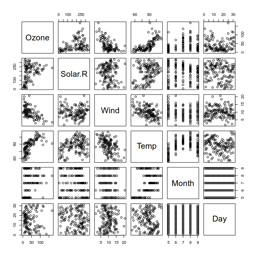
One of the nice features of plot() is that it produced plots based on the shape and type of data you give it.

To see this, let’s plot the data from the built in data frame airquality.

head(airquality)

A data.frame: 6 × 6

	Ozone	Solar.R	Wind	Temp	Month	Day
	<int>	<int>	<dbl>	<int>	<int>	<int>
1	41	190	7.4	67	5	1
2	36	118	8.0	72	5	2
3	12	149	12.6	74	5	3
4	18	313	11.5	62	5	4
5	NA	NA	14.3	56	5	5
6	28	NA	14.9	66	5	6

If we pass it the whole data frame, it produces a scatter plot lattice:

plot(airquality)

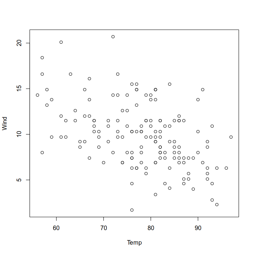
If we pass it just two columns, it produces a scatter plot:

plot(airquality[, c("Temp", "Wind")])

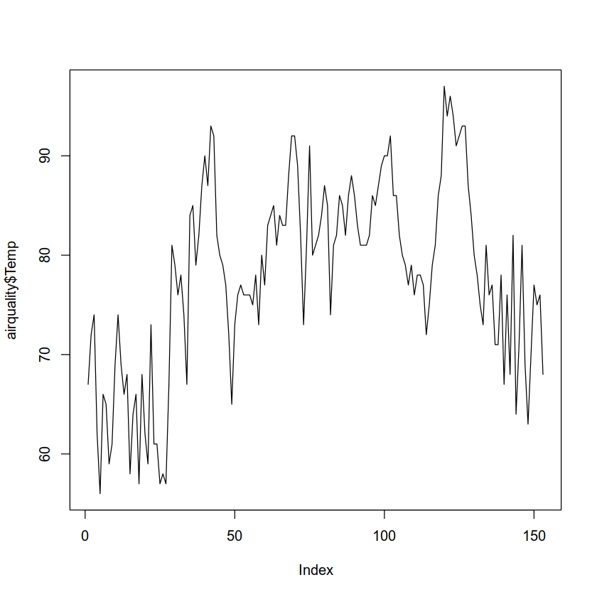
And if pass it one, it produces a line graph:

plot(airquality$Temp, type='l')

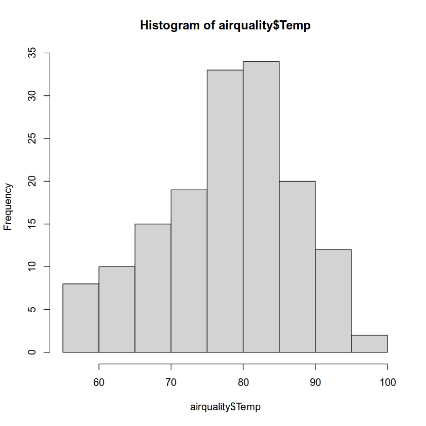
The hist() function will create a histogram:

hist(airquality$Temp)

Value Counts with table()

This function is like .value_counts() in Pandas.

It does a quick count of all the value types of a feature or combination of them.

Here we get a table of values and their counts for airquality$Month.

months <- table(airquality$Month)
months.df <- data.frame(months)
names(months.df) <- c("Month", "Freq")
t(months.df)

A matrix: 2 × 5 of type chr

Month	5	6	7	8	9
Freq	31	30	31	31	30

Note we used t() to transpose the data frame.