Programming for Data Science
Let’s explore Pandas in more depth using the Iris dataset.
This is a well-known demonstration dataset produced by R.A. Fischer, a notable figure in the history of statistics.
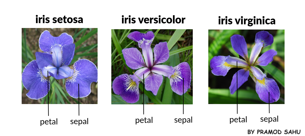
This dataset contains \(150\) observations on four features for three types of iris.
Load Iris Dataset
We’ll grab the dataset from the Seaborn visualization package.
The function load_dataset() in seaborn loads the built-in dataset.
import pandas as pdimport numpy as npimport seaborn as sns= sns.load_dataset('iris' )
0
5.1
3.5
1.4
0.2
setosa
1
4.9
3.0
1.4
0.2
setosa
2
4.7
3.2
1.3
0.2
setosa
3
4.6
3.1
1.5
0.2
setosa
4
5.0
3.6
1.4
0.2
setosa
...
...
...
...
...
...
145
6.7
3.0
5.2
2.3
virginica
146
6.3
2.5
5.0
1.9
virginica
147
6.5
3.0
5.2
2.0
virginica
148
6.2
3.4
5.4
2.3
virginica
149
5.9
3.0
5.1
1.8
virginica
150 rows × 5 columns
Heads and Tails
We can quickly inspect the data with .head() and .tail().
As we saw with Series, .head() returns the first \(5\) rows and .tail() the last.
0
5.1
3.5
1.4
0.2
setosa
1
4.9
3.0
1.4
0.2
setosa
2
4.7
3.2
1.3
0.2
setosa
3
4.6
3.1
1.5
0.2
setosa
4
5.0
3.6
1.4
0.2
setosa
145
6.7
3.0
5.2
2.3
virginica
146
6.3
2.5
5.0
1.9
virginica
147
6.5
3.0
5.2
2.0
virginica
148
6.2
3.4
5.4
2.3
virginica
149
5.9
3.0
5.1
1.8
virginica
You can return fewer or more rows by passing a different positive integer to these methods, e.g. .head(10).
0
5.1
3.5
1.4
0.2
setosa
1
4.9
3.0
1.4
0.2
setosa
2
4.7
3.2
1.3
0.2
setosa
3
4.6
3.1
1.5
0.2
setosa
4
5.0
3.6
1.4
0.2
setosa
5
5.4
3.9
1.7
0.4
setosa
6
4.6
3.4
1.4
0.3
setosa
7
5.0
3.4
1.5
0.2
setosa
8
4.4
2.9
1.4
0.2
setosa
9
4.9
3.1
1.5
0.1
setosa
Naming Indexes
We can name indexes, which is important to do in many cases.
= 'obs_id' # Each observation is a unique plant
obs_id
0
5.1
3.5
1.4
0.2
setosa
1
4.9
3.0
1.4
0.2
setosa
2
4.7
3.2
1.3
0.2
setosa
3
4.6
3.1
1.5
0.2
setosa
4
5.0
3.6
1.4
0.2
setosa
...
...
...
...
...
...
145
6.7
3.0
5.2
2.3
virginica
146
6.3
2.5
5.0
1.9
virginica
147
6.5
3.0
5.2
2.0
virginica
148
6.2
3.4
5.4
2.3
virginica
149
5.9
3.0
5.1
1.8
virginica
150 rows × 5 columns
Using a MultiIndex
We can also redefine indexes to reflect the logic of our data .
In this data set, the species of the flower is part of its identity , so it can be part of the index.
The other features vary by individual.
Note that species is also a label that can be used for training a model to predict the species of an iris flower. In that use case, the column would be pulled out into a separate vector.
= iris.reset_index().set_index(['species' ,'obs_id' ])
species
obs_id
setosa
39
5.1
3.4
1.5
0.2
versicolor
82
5.8
2.7
3.9
1.2
virginica
124
6.7
3.3
5.7
2.1
setosa
10
5.4
3.7
1.5
0.2
41
4.5
2.3
1.3
0.3
virginica
117
7.7
3.8
6.7
2.2
versicolor
89
5.5
2.5
4.0
1.3
virginica
123
6.3
2.7
4.9
1.8
setosa
4
5.0
3.6
1.4
0.2
versicolor
65
6.7
3.1
4.4
1.4
Row Selection (Filtering)
.iloc[]You can extract rows using indexes with .iloc[].
This works by indexing rows by their numeric sequence value.
This fetches row 3, and all columns.
sepal_length       4.7
sepal_width        3.2
petal_length       1.3
petal_width        0.2
species         setosa
Name: 2, dtype: object
We can use a slice to fetch rows with indices 1 and 2 (the right endpoint is exclusive), and all columns.
obs_id
1
4.9
3.0
1.4
0.2
setosa
2
4.7
3.2
1.3
0.2
setosa
Combining Filtering and Selecting
Recall the comma notation from NumPy — it is used here, too.
The first element is a row selector , the second a column selector .
In database terminology, row selection is called filtering.
Here we fetch rows 1 and 2 with and first three columns.
obs_id
1
4.9
3.0
1.4
2
4.7
3.2
1.3
.loc[]Filtering can also be done with .loc[].
This uses the row names and column names.
Here we ask for rows with labels 1, 2, and 3.
Note the slice returns the row with obs_id 3.
.iloc[] would return rows with indices 1, 2.
obs_id
1
4.9
3.0
1.4
0.2
setosa
2
4.7
3.2
1.3
0.2
setosa
3
4.6
3.1
1.5
0.2
setosa
1 :3 , ['sepal_width' ,'sepal_length' ]]
obs_id
1
3.0
4.9
2
3.2
4.7
3
3.1
4.6
The different behavior of the slice with .loc, 1:3 is due to the fact that it is short-hand for [1,2,3], a list of labels, not a range of offsets.
obs_id
1
4.9
3.0
1.4
0.2
setosa
2
4.7
3.2
1.3
0.2
setosa
3
4.6
3.1
1.5
0.2
setosa
So, for example, since there is no label value -1, this won’t work:
Here we subset on columns with column names as a list of strings:
1 :3 , ['sepal_length' ,'petal_width' ]]
obs_id
1
4.9
0.2
2
4.7
0.2
3
4.6
0.2
Here we select all rows, specific columns:
'sepal_length' ,'petal_width' ]]
obs_id
0
5.1
0.2
1
4.9
0.2
2
4.7
0.2
3
4.6
0.2
4
5.0
0.2
...
...
...
145
6.7
2.3
146
6.3
1.9
147
6.5
2.0
148
6.2
2.3
149
5.9
1.8
150 rows × 2 columns
That is same as this:
'sepal_length' ,'petal_width' ]]
obs_id
0
5.1
0.2
1
4.9
0.2
2
4.7
0.2
3
4.6
0.2
4
5.0
0.2
...
...
...
145
6.7
2.3
146
6.3
1.9
147
6.5
2.0
148
6.2
2.3
149
5.9
1.8
150 rows × 2 columns
We can use .loc[] with a MultiIndex, too.
Recall our DataFrame with a two element index:
species
obs_id
setosa
0
5.1
3.5
1.4
0.2
1
4.9
3.0
1.4
0.2
2
4.7
3.2
1.3
0.2
3
4.6
3.1
1.5
0.2
4
5.0
3.6
1.4
0.2
...
...
...
...
...
...
virginica
145
6.7
3.0
5.2
2.3
146
6.3
2.5
5.0
1.9
147
6.5
3.0
5.2
2.0
148
6.2
3.4
5.4
2.3
149
5.9
3.0
5.1
1.8
150 rows × 4 columns
We can select a single observation by its key, i.e. full label, expressed as a tuple:
'setosa' ,0 )]
sepal_length    5.1
sepal_width     3.5
petal_length    1.4
petal_width     0.2
Name: (setosa, 0), dtype: float64
We may also select all the setosas by using the first index column:
'setosa' ].head()
obs_id
0
5.1
3.5
1.4
0.2
1
4.9
3.0
1.4
0.2
2
4.7
3.2
1.3
0.2
3
4.6
3.1
1.5
0.2
4
5.0
3.6
1.4
0.2
Here we grab one species and one feature:
'setosa' , 'sepal_length' ].head()
obs_id
0    5.1
1    4.9
2    4.7
3    4.6
4    5.0
Name: sepal_length, dtype: float64
Note that this returns a Series.
If we want a DataFrame back, we can use .to_frame():
'setosa' , 'sepal_length' ].to_frame().head()
obs_id
0
5.1
1
4.9
2
4.7
3
4.6
4
5.0
Or we might pass a list instead of a string for the column selector:
'setosa' , ['sepal_length' ]].head()
obs_id
0
5.1
1
4.9
2
4.7
3
4.6
4
5.0
We use a tuple to index multiple index levels.
'setosa' , 5 )]
sepal_length    5.4
sepal_width     3.9
petal_length    1.7
petal_width     0.4
Name: (setosa, 5), dtype: float64
Or a list to get multiple rows, a la fancy indexing.
'setosa' ,'virginica' ]]
species
obs_id
setosa
0
5.1
3.5
1.4
0.2
1
4.9
3.0
1.4
0.2
2
4.7
3.2
1.3
0.2
3
4.6
3.1
1.5
0.2
4
5.0
3.6
1.4
0.2
...
...
...
...
...
...
virginica
145
6.7
3.0
5.2
2.3
146
6.3
2.5
5.0
1.9
147
6.5
3.0
5.2
2.0
148
6.2
3.4
5.4
2.3
149
5.9
3.0
5.1
1.8
100 rows × 4 columns
Boolean Indexing
It’s very common to subset a DataFrame based on some condition on the data.
Note that even though we are filtering rows, we are not using .loc[] or .iloc[] here.
Pandas knows what to do if you pass a boolean structure.
Here is a boolean Series.
obs_id
0      False
1      False
2      False
3      False
4      False
       ...
145    False
146    False
147    False
148    False
149    False
Name: sepal_length, Length: 150, dtype: bool
We can pass it to the DataFrame to select the True rows:
>= 7.5 ]
obs_id
105
7.6
3.0
6.6
2.1
virginica
117
7.7
3.8
6.7
2.2
virginica
118
7.7
2.6
6.9
2.3
virginica
122
7.7
2.8
6.7
2.0
virginica
131
7.9
3.8
6.4
2.0
virginica
135
7.7
3.0
6.1
2.3
virginica
And we may combine boolean expressions, too, making sure we group things with parentheses.
>= 4.5 ) & (iris.sepal_length <= 4.7 )]
obs_id
2
4.7
3.2
1.3
0.2
setosa
3
4.6
3.1
1.5
0.2
setosa
6
4.6
3.4
1.4
0.3
setosa
22
4.6
3.6
1.0
0.2
setosa
29
4.7
3.2
1.6
0.2
setosa
41
4.5
2.3
1.3
0.3
setosa
47
4.6
3.2
1.4
0.2
setosa
And here we add a column selection.
>= 4.5 ) & (iris.sepal_length <= 4.7 ), ['sepal_length' ]]
obs_id
2
4.7
3
4.6
6
4.6
22
4.6
29
4.7
41
4.5
47
4.6
Working with Missing Data
Pandas primarily uses the data type np.nan from NumPy to represent missing data.
= pd.DataFrame({'x' : [2 , np.nan, 1 ], 'y' : [np.nan, np.nan, 6 ]}
These values appear as NaNs:
0
2.0
NaN
1
NaN
NaN
2
1.0
6.0
.dropna()We can drop all rows with missing data in any column using dropna().
= df_miss.dropna()
The subset parameter takes a list of column names to specify which columns should have missing values.
= df_miss.dropna(subset= ['x' ])
.fillna()This will replace missing values with whatever you set it to, e.g. \(0\) s.
We can pass the results of an operation — for example to peform simple imputation , we can replace missing values in each column with the median value of the respective column:
= df_miss.fillna(df_miss.median())
0
2.0
6.0
1
1.5
6.0
2
1.0
6.0
Sorting
.sort_values()We use .sort_values() to sort the data in a DataFrame.
The by parameter takes string or list of strings, defining the columns and order to sort on.
The ascending parameter takes True or False. This may be a list if you want diffferent sort order for different columns.
And the inplace paramter takes True or False.
= ['sepal_length' ,'petal_width' ], ascending= False ).head(10 )
obs_id
131
7.9
3.8
6.4
2.0
virginica
118
7.7
2.6
6.9
2.3
virginica
135
7.7
3.0
6.1
2.3
virginica
117
7.7
3.8
6.7
2.2
virginica
122
7.7
2.8
6.7
2.0
virginica
105
7.6
3.0
6.6
2.1
virginica
130
7.4
2.8
6.1
1.9
virginica
107
7.3
2.9
6.3
1.8
virginica
109
7.2
3.6
6.1
2.5
virginica
125
7.2
3.2
6.0
1.8
virginica
.sort_index()Recall that indexes and data are accessed differently in Pandas.
To sort the index of a DataFrame, use this method.
= 0 , ascending= False )
obs_id
149
5.9
3.0
5.1
1.8
virginica
148
6.2
3.4
5.4
2.3
virginica
147
6.5
3.0
5.2
2.0
virginica
146
6.3
2.5
5.0
1.9
virginica
145
6.7
3.0
5.2
2.3
virginica
...
...
...
...
...
...
4
5.0
3.6
1.4
0.2
setosa
3
4.6
3.1
1.5
0.2
setosa
2
4.7
3.2
1.3
0.2
setosa
1
4.9
3.0
1.4
0.2
setosa
0
5.1
3.5
1.4
0.2
setosa
150 rows × 5 columns
Statistics
Pandas has a number of statistic operations built into it.
.describe()As we saw above, this method computes some basic statistics from the DataTable if applicable.
count
150.000000
150.000000
150.000000
150.000000
mean
5.843333
3.057333
3.758000
1.199333
std
0.828066
0.435866
1.765298
0.762238
min
4.300000
2.000000
1.000000
0.100000
25%
5.100000
2.800000
1.600000
0.300000
50%
5.800000
3.000000
4.350000
1.300000
75%
6.400000
3.300000
5.100000
1.800000
max
7.900000
4.400000
6.900000
2.500000
We can transpose this for easier reading:
sepal_length
150.0
5.843333
0.828066
4.3
5.1
5.80
6.4
7.9
sepal_width
150.0
3.057333
0.435866
2.0
2.8
3.00
3.3
4.4
petal_length
150.0
3.758000
1.765298
1.0
1.6
4.35
5.1
6.9
petal_width
150.0
1.199333
0.762238
0.1
0.3
1.30
1.8
2.5
We can also call it on a single feature, i.e. a Series.
Notice the difference between a column of strings and one of numbers.
count        150
unique         3
top       setosa
freq          50
Name: species, dtype: object
count    150.000000
mean       5.843333
std        0.828066
min        4.300000
25%        5.100000
50%        5.800000
75%        6.400000
max        7.900000
Name: sepal_length, dtype: float64
.value_counts()This is a highly useful function for showing the frequency for each distinct value in a column.
species
setosa        50
versicolor    50
virginica     50
Name: count, dtype: int64
We can also extract a new table for the distinct values of a column.
= iris.species.value_counts().to_frame('n' )
species
setosa
50
versicolor
50
virginica
50
We can show relative frequency instead of counts:
= True )
species
setosa        0.333333
versicolor    0.333333
virginica     0.333333
Name: proportion, dtype: float64
The method returns a Series that can be converted into a DataFrame.
= iris.sepal_length.value_counts().to_frame('n' )
sepal_length
5.0
10
5.1
9
6.3
9
5.7
8
6.7
8
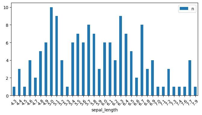
You can run .value_counts() on a column to get a kind of histogram:
= (8 ,4 ), rot= 45 );
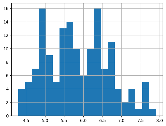
You can see that this method produces similar results to a histogram:
= 20 );
.mean()Statistical properties are easily computed.
Operations like this generally exclude missing data.
So, it is import to convert missing data to values if they need to be considered in the denominator.
.std()This standard deviation.
.corr()We may get the correlations among features with .corr():
# iris.corr() # Won't work because of string column
= True , method= 'pearson' )
sepal_length
1.000000
-0.117570
0.871754
0.817941
sepal_width
-0.117570
1.000000
-0.428440
-0.366126
petal_length
0.871754
-0.428440
1.000000
0.962865
petal_width
0.817941
-0.366126
0.962865
1.000000
# This works because we moved the string into the index
sepal_length
1.000000
-0.117570
0.871754
0.817941
sepal_width
-0.117570
1.000000
-0.428440
-0.366126
petal_length
0.871754
-0.428440
1.000000
0.962865
petal_width
0.817941
-0.366126
0.962865
1.000000
Note that the method parameter defaults to pearson.
You may also use spearman, kendall, or a custom function.
Correlation can be computed on two columns, or features, by subsetting on them:
'sepal_length' ,'petal_length' ]].corr()
sepal_length
1.000000
0.871754
petal_length
0.871754
1.000000
Here we correlate three features:
'sepal_length' ,'petal_length' ,'sepal_width' ]].corr()
sepal_length
1.000000
0.871754
-0.11757
petal_length
0.871754
1.000000
-0.42844
sepal_width
-0.117570
-0.428440
1.00000
Styling
Pandas provides methods for styling DataFrames as quick way to visualize data.
= True ).style.background_gradient(cmap= "Blues" , axis= None )
sepal_length
1.000000
-0.117570
0.871754
0.817941
sepal_width
-0.117570
1.000000
-0.428440
-0.366126
petal_length
0.871754
-0.428440
1.000000
0.962865
petal_width
0.817941
-0.366126
0.962865
1.000000
Visualization with .plot()
The .plot() method allows for quick visualizations such as scatterplots, bar charts, and histograms.
We will cover visualization separately in more detail.
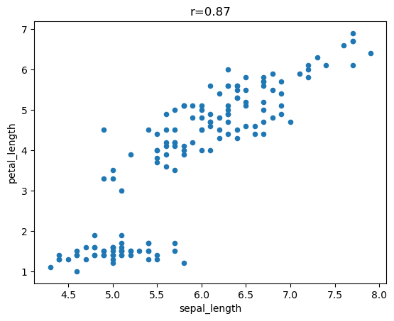
= ['sepal_length' , 'petal_length' ]= f"r= { round (iris[features].corr().iloc[0 ,1 ], 2 )} " * my_features, title= my_title);
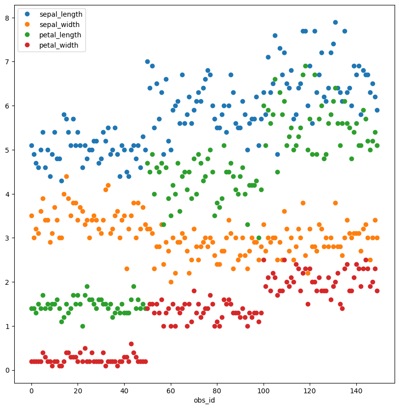
Here we plot all the data as points.
Note how .plot() color codes the features for us.
list (iris.columns)).plot(style= 'o' , figsize= (10 ,10 ));
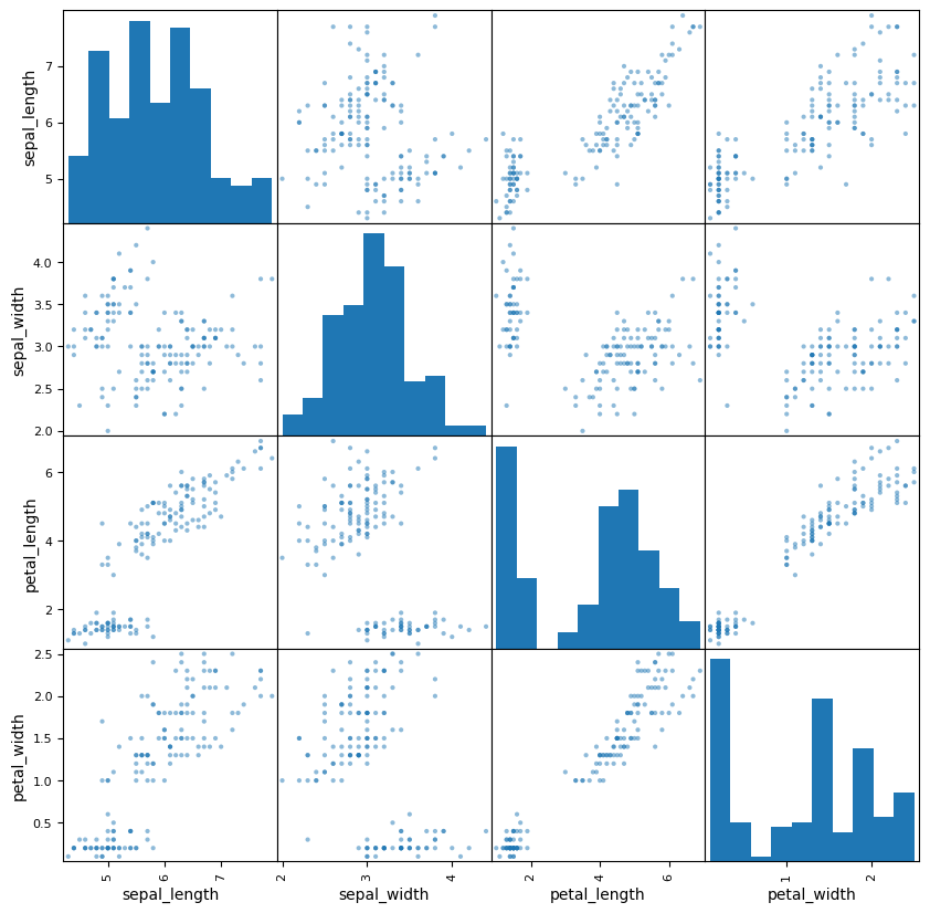
Here we use Seaborn’s scatter matrix function.
from pandas.plotting import scatter_matrix
= (10 ,10 ));
Saving to a CSV File
It is common practice to save a DataFrame to a CSV file.
Use .to_csv() for this.
'./iris_data.csv' , index= True )
There are also options to save to a database, other file formats, even the clipboard.
A file path is required; it will create the file if it does not exist, or overwrite it if it does.
You may also append by passing a to the mode parameter.
Other optional parameters include:
sep: to set the delimiter to something other than a comma, e.g. a pipe | or tab \t.
index: to save the index column(s) or not.
Reading from a CSV File
.read_csv() reads from CSV into DataFrame
= pd.read_csv('./iris_data.csv' ).set_index('obs_id' )
obs_id
0
setosa
5.1
3.5
1.4
0.2
1
setosa
4.9
3.0
1.4
0.2
2
setosa
4.7
3.2
1.3
0.2
3
setosa
4.6
3.1
1.5
0.2
4
setosa
5.0
3.6
1.4
0.2
Note we apply the .set_index() method immediately.
